Standalone ANS Labelling Tool

About this guide

This guide walks new users through the ANS Labelling Tool from the very first launch through completing a fully annotated dataset. No prior experience with image labelling tools is assumed.

It is written for data scientists, annotators, and team leads who are preparing image datasets for computer-vision models — object detection, instance segmentation, or oriented bounding boxes (OBB).

Conventions used throughout this guide:

• Menu paths are written as “File → Open Dataset…”.
• Keyboard shortcuts use macOS notation (⌘ = Command, ⇧ = Shift). On Windows and Linux, replace ⌘ with Ctrl.
• Buttons and on-screen labels appear in bold, e.g. Sign In.
• Screenshots are taken on macOS. The layout is identical on Windows and Linux.

1. Introduction

The ANS Labelling Tool is a desktop application for creating high-quality image datasets for computer-vision training. It supports three annotation tasks — rectangular bounding boxes for object detection, polygons for instance segmentation, and rotated bounding boxes (OBB) for objects that do not align with image axes — and reads and writes the open-source “ANS standard format”, which is a flat folder of images with sidecar text label files plus an ANS_Class.json class definition.

It can also import datasets in many popular third-party formats (YOLO, COCO, Pascal VOC, CreateML, Paligemma, Darknet and more), automatically converting them into the ANS format while keeping the original folder intact.

1.1 Key features

• Three annotation modes — detection (box), segmentation (polygon), and OBB (oriented box).
• AI-assisted Auto-segment and Auto-label that pre-populate labels you only need to verify.
• One-click import of YOLO, COCO, Pascal VOC, CreateML, Paligemma, Darknet, TFRecord and more.
• Per-image and dataset-wide class statistics with class-balance percentages.
• Built-in image augmentation (rotation, flip, brightness, contrast and more).
• Multi-language UI — English, Vietnamese, Spanish, Japanese.
• Undo/redo for every label edit; copy-paste labels between images.
• Available for macOS (Apple Silicon and Intel), Windows 10/11, and Linux (AppImage).

1.2 System requirements

• macOS 12 Monterey or later (Apple Silicon recommended), or Windows 10/11, or any modern Linux distribution with FUSE installed.
• 8 GB RAM minimum, 16 GB recommended for large datasets.
• Optional: NVIDIA GPU with current driver and CUDA for the fastest Auto-segment / Auto-label.
• An ANSCENTER account — sign up free at https://portal.anscenter.com.au.
• Network connection (sign-in only — labelling itself is fully offline).

2. Installation

Download the Standalone ANS Labelling Tool from the ANS Portal before you launch it for the first time.

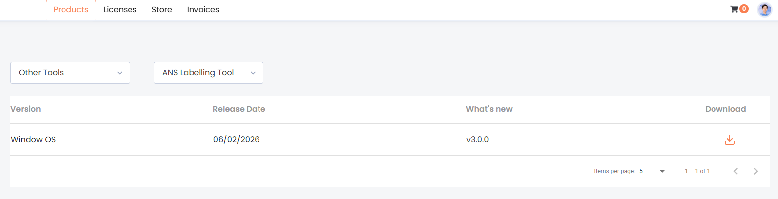
Figure: ANS Labelling Tool download page in ANS Portal.

1. Sign in to the ANS Portal.
2. Go to Products.
3. Select Other Tools from the product category drop-down list.
4. Select ANS Labelling Tool from the tool drop-down list.
5. In the Download column, click the download icon for the available installer.
6. Run the downloaded installer and follow the on-screen instructions.

3. First launch

The first time you open the app you will see the sign-in screen. Once you sign in, the app asks you to pick the annotation task you want to start with, then drops you into the main labelling workspace.

3.1 Signing in

Use the credentials issued by your ANSCENTER account. If your team admin gave you a username and a temporary password, sign in once and then change the password in the ANSCENTER portal.

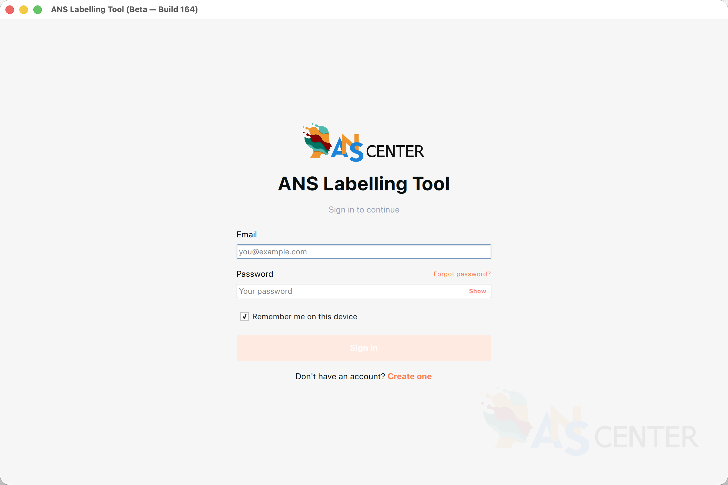
Figure: The sign-in screen on first launch.

1. Type your email address in the Email field.
2. Type your password in the Password field. Click Show to reveal what you typed if you want to double-check.
3. Leave Remember me on this device ticked if you trust this computer — the app will silently restore your session next time you launch it.
4. Click Sign In or press Return.

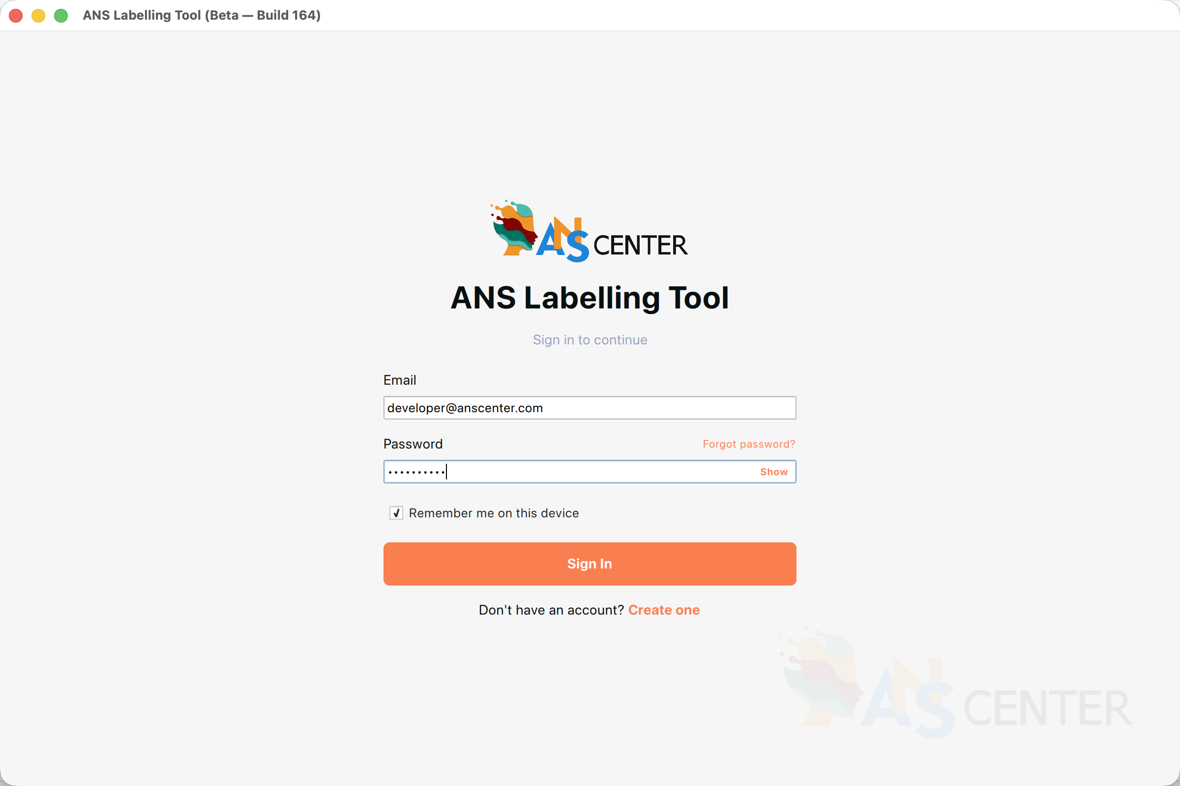
Figure: The form with credentials filled in. The Sign In button enables once both fields are non-empty.

tip

forgot your password? Use Forgot password? on the form — it opens the ANSCENTER portal in your browser where you can reset it. The labelling app itself does not change passwords.

3.2 Creating an account

If you do not yet have an ANSCENTER account, click Create one on the login screen. The registration form asks for your full name, phone number, email and a password. New accounts may need to be approved by your team admin before they can sign in.

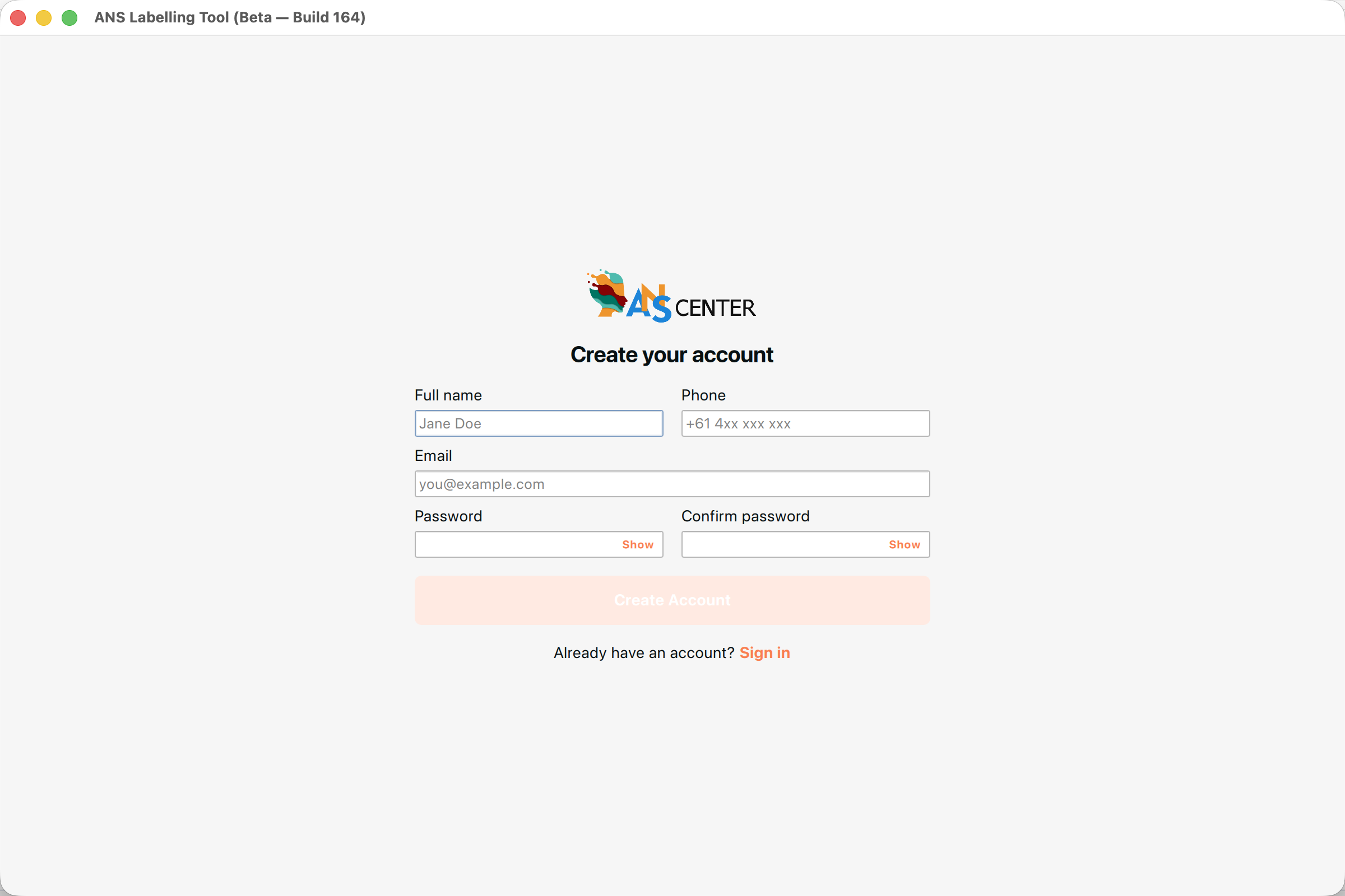
Figure: Account creation screen — reached via Create one on the login screen.

1. Click Create one at the bottom of the login screen.
2. Fill in Full name, Phone, Email, Password and Confirm password.
3. Click Create Account.
4. If your account requires manual approval, you will see a notice and be returned to the login screen — sign in once the admin approves you.

3.3 Choosing your annotation task

After the first successful sign-in the app asks which annotation task you want to start with. The choice is per user and is remembered between sessions; you can change it any time from File → Switch task…

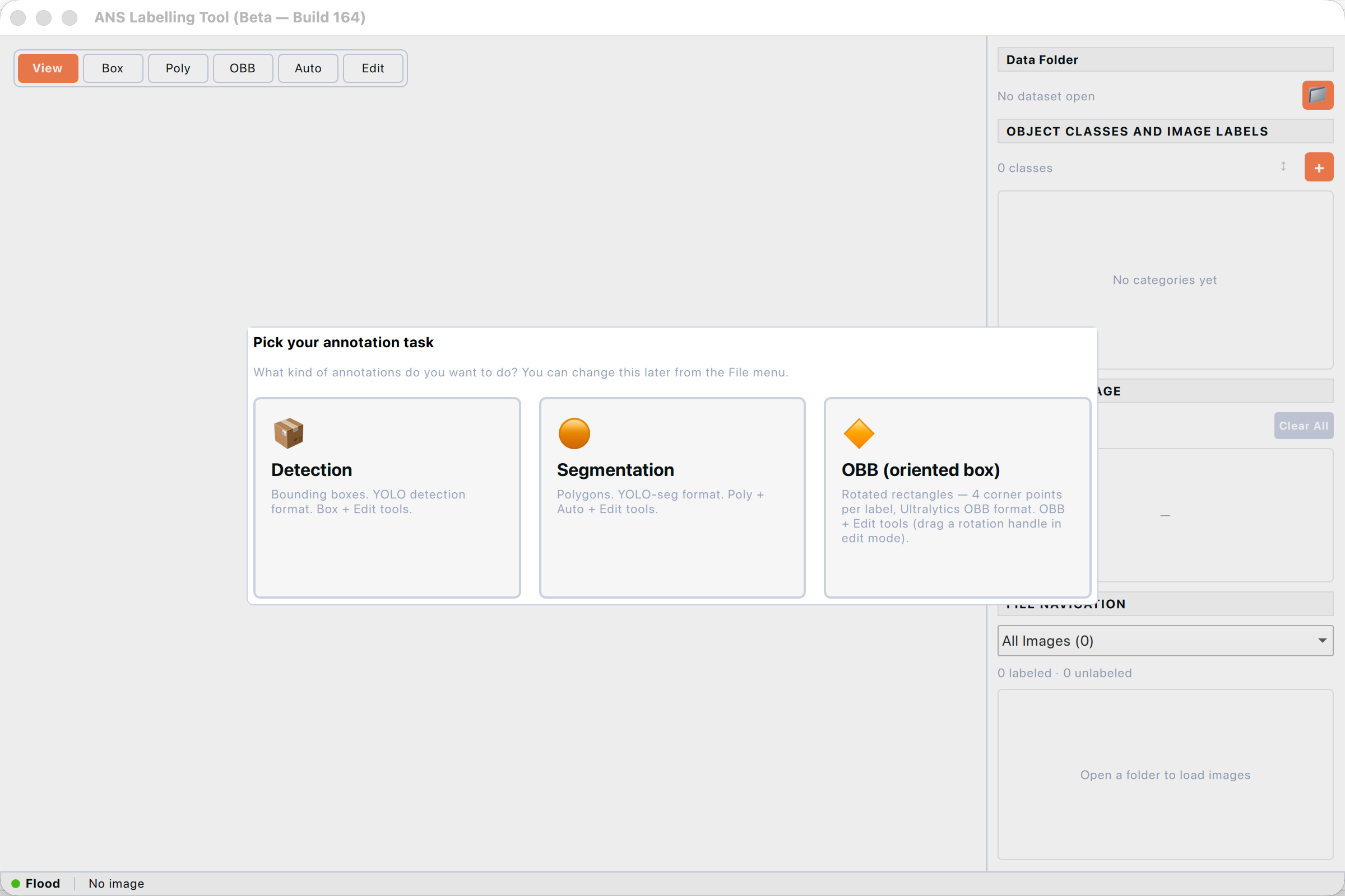
Figure: First-launch task picker. Click a card to choose your annotation task.

Click the card that matches your work. The dialog closes and the matching toolbar appears.

• Detection — rectangular bounding boxes. Best for objects that fit a rectangle (vehicles, products, people).
• Segmentation — polygons that trace the exact outline of the object. Best for irregular shapes or when you need pixel-accurate masks.
• OBB (oriented box) — rotated rectangles with four corner points. Best for elongated objects that lie at an angle (text on receipts, bricks, ships from above).

You can switch tasks later without losing any data — each task keeps its own most-recent dataset folder.

4. The workspace at a glance

After signing in and choosing a task, the labelling workspace fills the window. It is split into three vertical regions: the tool toolbar on the left, the canvas in the centre, and a control panel on the right.

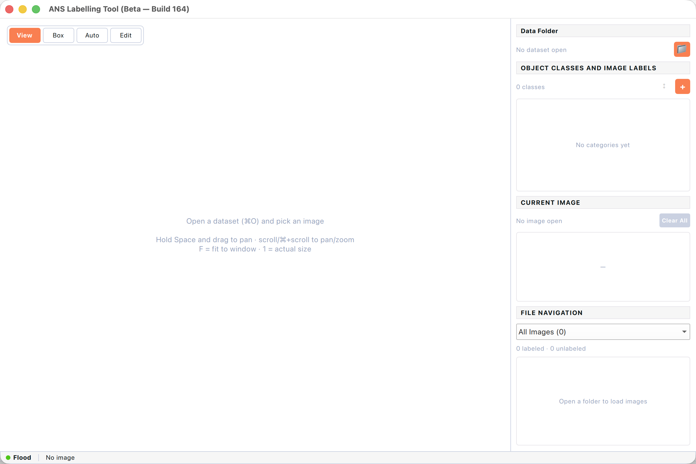
Figure: Empty workspace immediately after first sign-in — no dataset is open yet.

4.1 Window layout

The right-hand panel contains four collapsible sections, from top to bottom:

• Data Folder — shows the currently open dataset path and a folder-picker icon to open another.
• Object Classes and Image Labels — the list of categories defined for this dataset, with per-class counts. Below it, the list of labels on the currently visible image.
• Current Image — the image dimensions plus a red Clear All button that removes every label on the current image (with a confirmation prompt).
• File Navigation — a drop-down to filter by All / Labeled / Unlabeled, a counter, and the scrollable file list. Green dots mark labeled files, grey dots mark unlabeled ones.

4.2 The tool toolbar

The buttons in the top-left corner of the canvas switch between tool modes. The set of buttons depends on your current task:

• View — pan with Space+drag, zoom with the scroll wheel. No drawing is possible in this mode.
• Box — draw a rectangular bounding box (Detection task only).
• Poly — draw a polygon vertex by vertex (Segmentation task only).
• OBB — draw a rotated rectangle by dragging, then adjust the rotation handle in Edit mode (OBB task only).
• Auto — AI-assisted Auto-segment. Hover over an object to see a ghost preview and click to commit. Requires either the SAM/AI backend or the simple Flood-fill backend.
• Edit — select existing labels to move, resize, recolour or delete them.

4.3 Zoom and pan

The zoom badge in the top-right corner of the canvas shows the current zoom percentage. To pan and zoom:

• Hold Space and drag — pan the image in any mode.
• ⌘ + scroll wheel — zoom in / out centred on the cursor.
• Scroll wheel alone — pan vertically; ⇧ + scroll — pan horizontally.
• F — fit the image to the canvas. 1 — reset to actual size (100%).
• ⌘= / ⌘− — zoom in / out from the centre.

4.4 Status bar

The thin grey strip at the very bottom of the window summarises what the app is doing: the active Auto backend (AI or Flood), the current file name and dimensions, the position in the dataset, the per-class label count for the current image, and a small spinner when a long-running operation (like converting a dataset) is in progress.

5. Opening and importing datasets

The labelling tool always works on a single dataset folder at a time. That folder must be in the ANS standard format — a flat directory of images and matching label files plus an ANS_Class.json that defines the categories.

5.1 The ANS standard format

An ANS dataset folder contains:

• Images in any of these formats: .jpg, .jpeg, .png, .bmp.
• One label sidecar per image with the same base filename and a .txt extension, e.g. cat01.jpg pairs with cat01.txt.
• A single ANS_Class.json at the root that lists every category: its ID, display name, colour, item count, and task type (detection / segmentation / obb).

Images without a matching .txt are considered unlabeled. The format is intentionally compatible with Ultralytics YOLO so you can train directly on the folder without further conversion.

5.2 Opening an existing dataset

To open an ANS-format dataset folder:

1. Choose File → Open Dataset… or press ⌘O.
2. Pick the folder that contains ANS_Class.json and the images. (Do not pick the parent — pick the actual folder of images.)
3. The first image is selected automatically. Use the file list on the right to jump to any image.

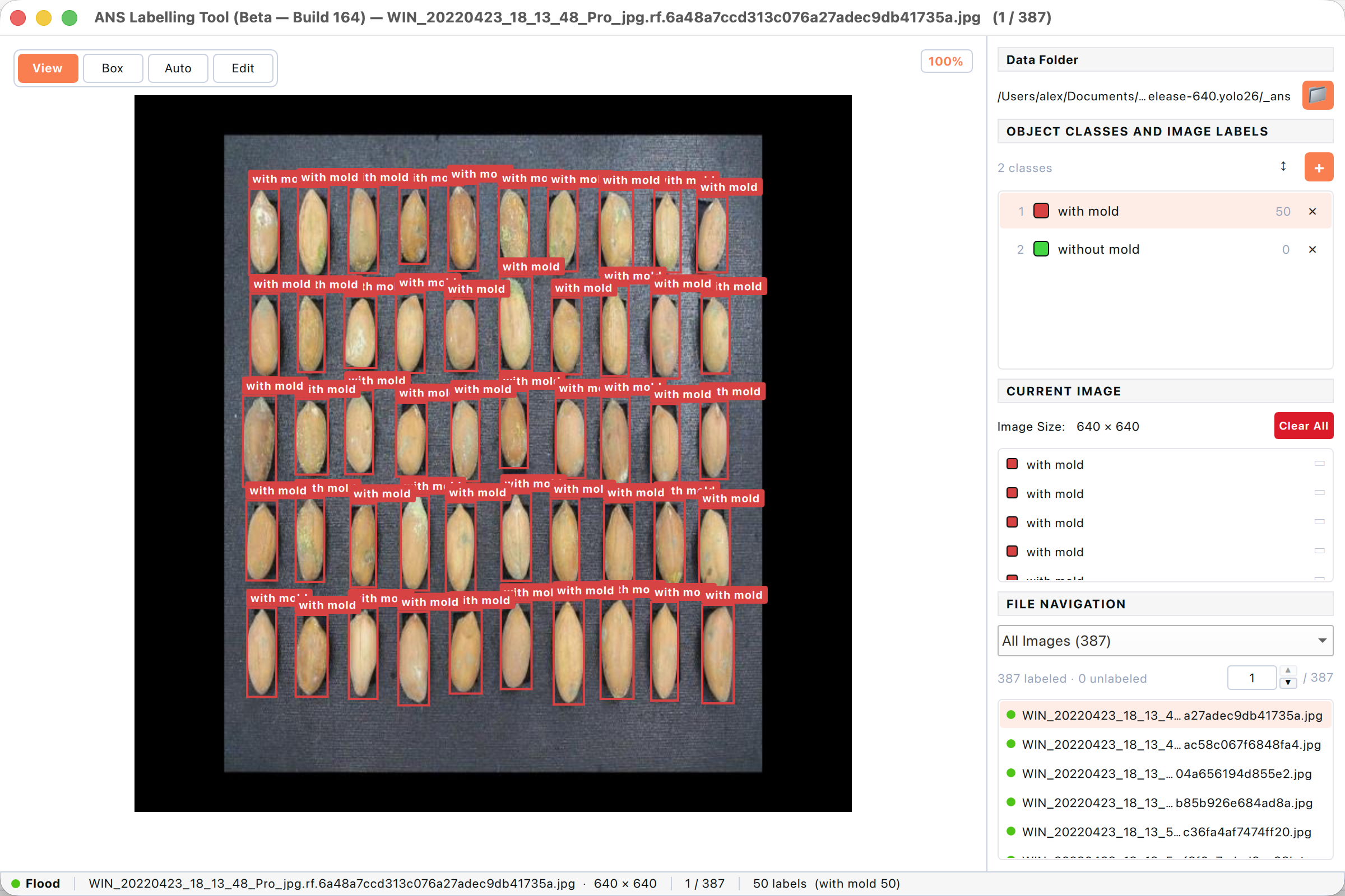
Figure: Detection task with a peanut quality-control dataset loaded.

Existing labels render on the canvas immediately. The category list on the right shows how many instances of each class have been drawn.

5.3 Importing a non-ANS dataset

If you open a folder that doesn’t already have ANS_Class.json, the tool detects the format and offers to convert it. This works for YOLO (detection, segmentation, OBB), COCO JSON, Pascal VOC XML, CreateML, Paligemma JSONL, Darknet, TFRecord and a few others.

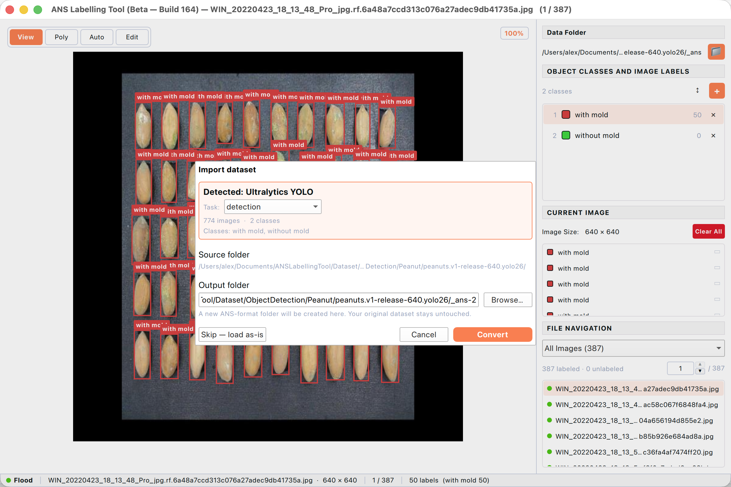
_Figure: Import dataset dialog. The tool auto-detects the source format and proposes a new ans folder.

1. Choose File → Open Dataset… and pick the original (non-ANS) folder. The Import dataset dialog appears.
2. Confirm the detected format and task. Adjust Task if the auto-detection is wrong.
3. Review the image count and the list of classes — these come from the source dataset’s class definition.
4. Either click Convert to create a sibling folder named _ans next to the source, or Skip — load as-is to read the source without converting.

note

Convert never modifies the original folder. The result is a brand-new _ans folder alongside it. You can keep your YOLO / COCO export untouched.

5.4 Supported source formats

The Convert step can read all of these:

• Ultralytics YOLOv5 / YOLOv7 / YOLOv8 / YOLOv9 / YOLOv11 / YOLOv12 / YOLO 26 (detection, segmentation, OBB).
• COCO JSON (detection, segmentation, keypoints).
• Pascal VOC XML.
• CreateML JSON.
• Google Paligemma JSONL.
• Darknet .txt with obj.names.
• TensorFlow TFRecord (detection).
• Florence-2 grounding format.
• Roboflow “Benchmarker” package.

6. Drawing labels

Each annotation task uses a different drawing tool, but the workflow is the same: pick a tool, draw the shape, then choose its category from the picker that pops up. You can always revert with ⌘Z.

6.1 Detection — bounding boxes

Use bounding boxes when the object fits inside a rectangle (cars, products on a shelf, faces, etc.). Each box is the tightest rectangle that fully contains the object.

1. Make sure you are in the Detection task. The toolbar shows View · Box · Auto · Edit.
2. Click Box (or press B) to enter draw mode. A crosshair follows the cursor.
3. Press and hold the left mouse button at one corner of the object, drag to the opposite corner, then release.
4. The category picker appears — choose the class. The box turns the class colour and a small label appears at the top.
5. Repeat for every visible object. Use F to fit and 1 to reset zoom if you lose track.

Figure: Drawn bounding boxes labelled “with mold” on a peanut image.

tip

hold ⇧ while drawing to constrain to a square. Box height and width must each be at least 3 pixels — anything smaller is silently dropped.

6.2 Segmentation — polygons

Use polygons when you need the exact outline of an object (clothing, road lanes, organs in medical images). Polygons are saved in YOLO-seg format.

1. Make sure you are in the Segmentation task. The toolbar shows View · Poly · Auto · Edit.
2. Click Poly (or press P) to enter draw mode.
3. Click once at a starting point on the object’s edge, then click around the contour adding one vertex at a time.
4. Close the polygon by double-clicking, right-clicking, or clicking back on the first vertex.
5. Choose the category in the picker that appears.
6. Press Escape at any time to cancel an in-progress polygon.

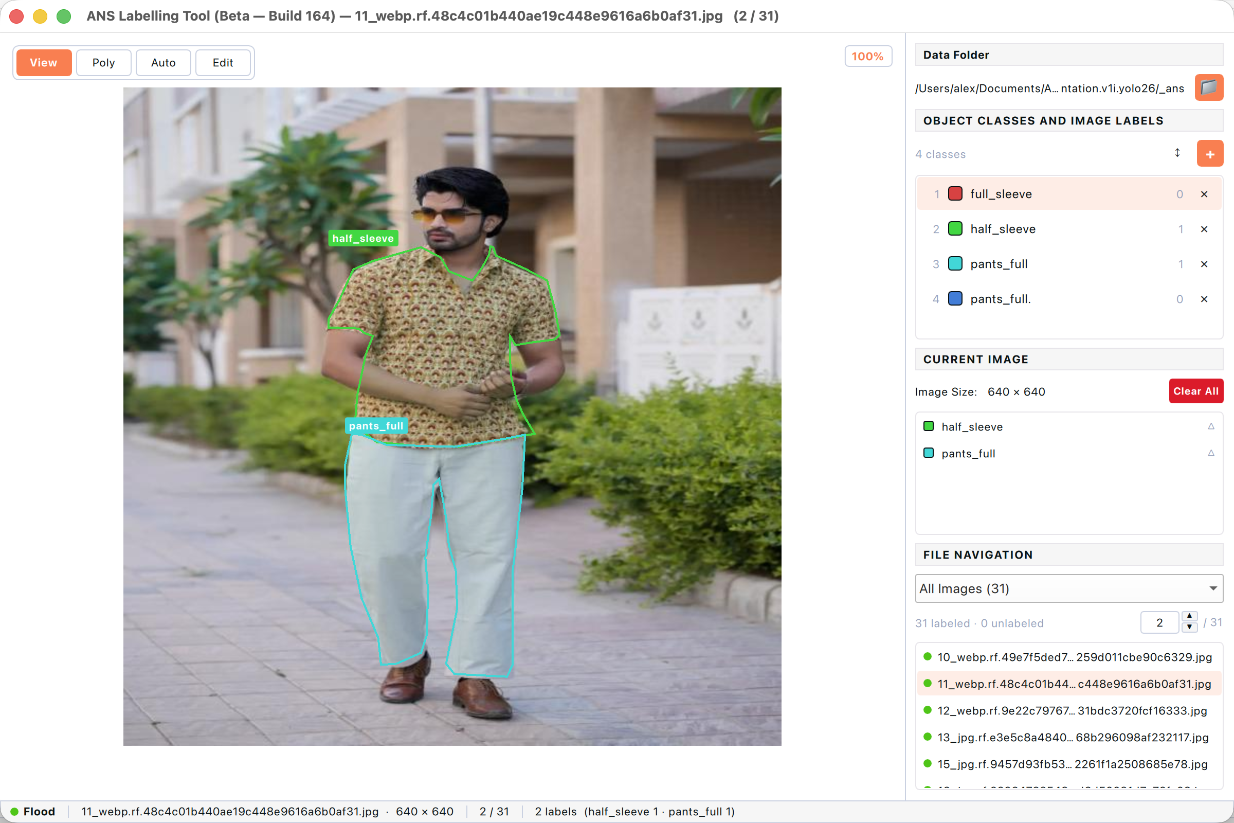
Figure: Polygon labels (half_sleeve, pants_full) traced around a person in a segmentation dataset.

tip

more vertices give a tighter outline but slow down training. 8–20 vertices is a good balance for most objects. Use Auto-segment for a head start — the AI will trace the outline and you only need to nudge a few vertices.

6.3 OBB — oriented bounding boxes

Use OBB when objects sit at an angle and a regular box would include too much background (angled bricks, aerial views of ships, text lines on a tilted receipt). OBB labels save the four rotated corner points in Ultralytics OBB format.

1. Switch to the OBB task. The toolbar shows View · OBB · Auto · Edit.
2. Click OBB (or press O) and drag a regular rectangle around the object.
3. After the category picker, switch to Edit mode (E) and grab the small rotation handle that appears at one end of the rectangle.
4. Drag the rotation handle to align the long side with the object.
5. Fine-tune the four corner points the same way as resizing a regular box.

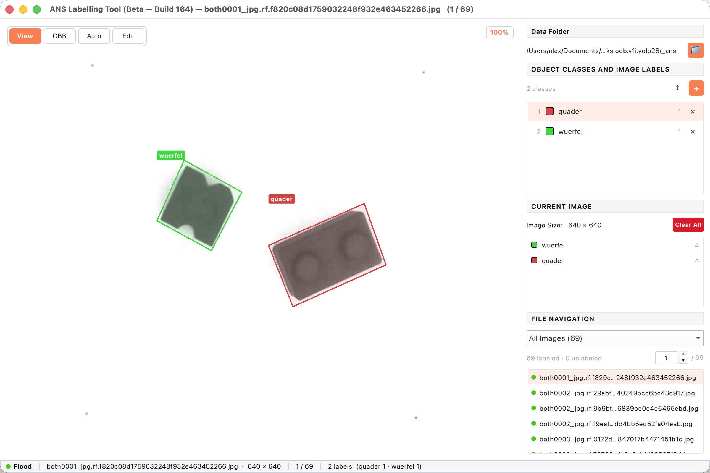
Figure: Rotated OBB labels around two bricks lying at an angle.

6.4 The label picker

After every shape you finish, a small menu pops up at the cursor with the list of categories. It always appears — there is no silent inheritance of the “current” class from the panel, so you can never mislabel by accident.

• Click a category name to commit the label.
• The category that was active in the right panel is shown in bold.
• The last entry is Add new category… — pick it to define a new class on the spot.
• Press Escape to discard the shape entirely.

If you enable Pick class on each Auto click under Display preferences, the picker also appears after every Auto-segment click. Turn it off to repeat the previous class without the prompt.

6.5 Editing existing labels

Click Edit (or press E) to switch to selection mode. The toolbar Edit button turns orange and resize handles appear on whichever label is selected. Edit mode is available in all three tasks and is the only way to delete or move existing labels.

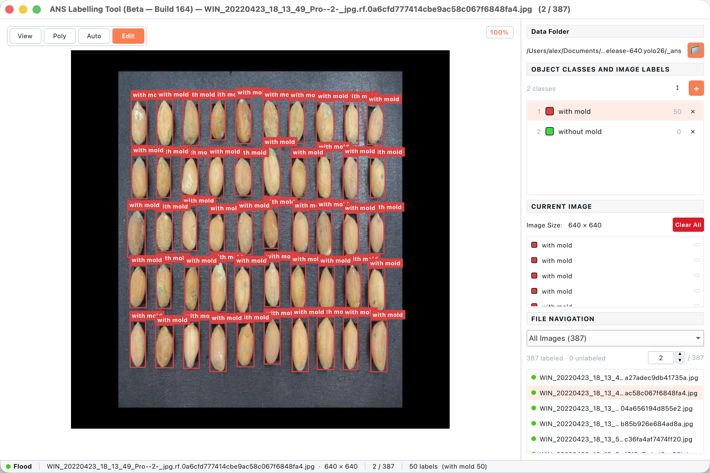
Figure: Edit mode active — the Edit button is highlighted, ready to select and modify labels.

• Click a label to select it. Hold ⇧ to add others to the selection.
• Drag the centre of a selected label to move it. Drag a corner handle to resize.
• For an OBB label, drag the small rotation handle to rotate it.
• Press Delete or ⌫ to remove every selected label (Undo with ⌘Z if you change your mind).
• Click the small × beside a class in the right panel to delete every label of that class on the current image.

6.6 Adding a new category

Categories can be added on the fly without leaving the canvas. The new class is appended to ANS_Class.json and immediately usable. The display colour is chosen randomly — change it later from the right-panel category row.

1. Draw any shape (box, polygon, OBB) — the label picker pops up.
2. Choose Add new category… at the bottom of the picker.
3. Type the category name. Names must be unique; duplicates are rejected with a message.
4. Click Ok. The shape commits with the new class, which now appears in the right-hand panel.

7. A worked example — labelling from scratch

This chapter walks through labelling a brand-new dataset end-to-end: opening a folder of images that has never been touched by the tool, creating a category, drawing the first few boxes, and saving the result. Follow along with any folder of your own .jpg / .png images to learn the rhythm.

7.1 Open an unlabelled folder

Use File → Open Dataset… (⌘O) and pick a folder that contains only image files — no ANS_Class.json, no .txt sidecars. The app opens it directly because nothing needs converting; you simply see an empty workspace ready for you to start.

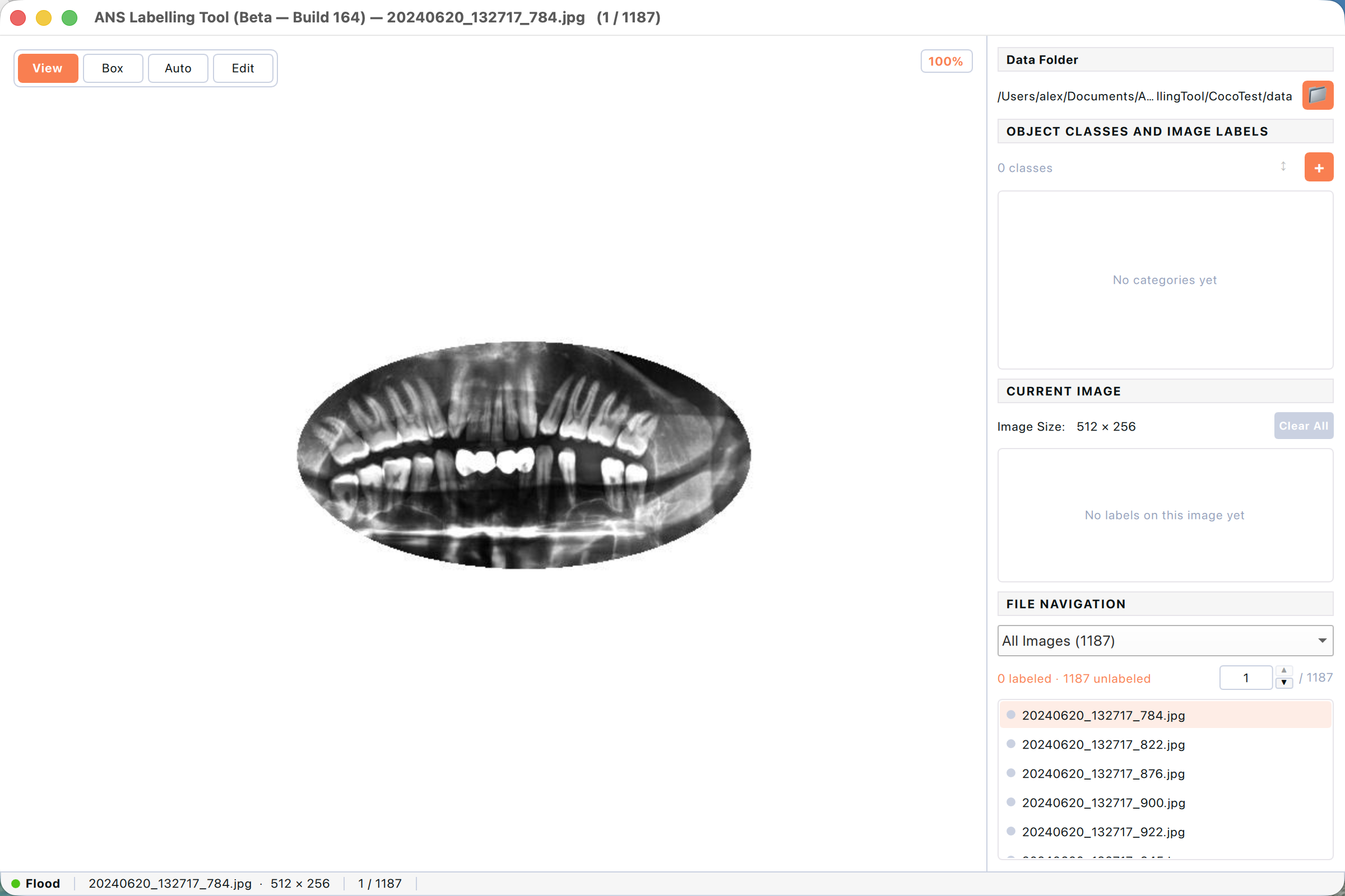
Figure: A freshly opened folder with no annotations. The right panel reports “0 classes / No categories yet” and “0 labeled · N unlabeled”.

The first image is selected automatically. Notice the right-hand panel — it reads “0 classes”, “No categories yet”, and the file list shows every image with a grey dot (unlabelled). Before drawing anything, you need at least one category.

7.2 Create your first category

There are two ways to add a category. The first is from the right-panel header — useful when you want to plan your taxonomy before drawing anything. (The second, “add on the fly” from the label picker, is shown in §6.3.)

1. Click the orange + button in the top-right of the Object Classes and Image Labels header.
2. An Add category dialog appears with a Name field.
3. Type the category name (it must be unique across this dataset).
4. Click Ok or press Return. The category is appended to ANS_Class.json with a randomly chosen colour and ID 1.

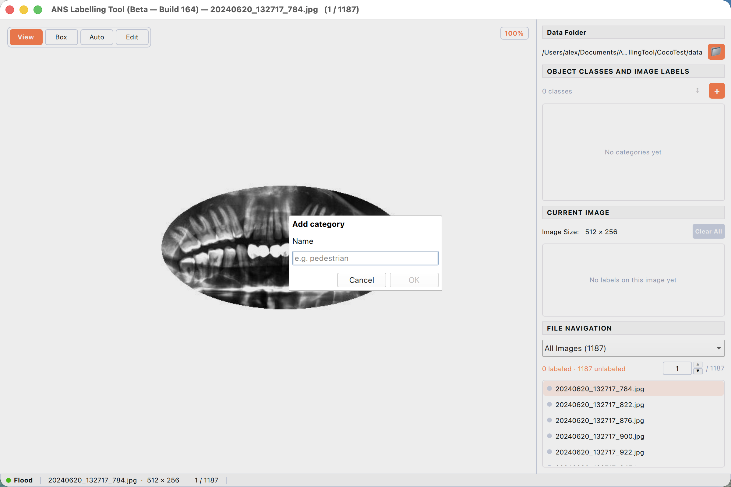
Figure: The Add category dialog with the Name field empty.

Figure: Typing a category name. The Ok button enables once the field has content.

Figure: After Ok, the new category appears in the right panel with a coloured swatch and a class index.

7.3 Draw the first labels

With at least one category defined, you can switch to draw mode and start labelling. In Detection task the draw tool is Box (shortcut B); in Segmentation it is Poly (P); in OBB it is OBB (O). The picker pop-up logic is identical for all three.

1. Click Box (or press B) — the cursor becomes a crosshair.
2. Press and hold the left mouse button at one corner of the object, drag to the opposite corner, and release.
3. The label picker appears at the cursor. It always shows two things — “+ Add new category…” at the top, and every existing category below.
4. Click your category. The box turns the class colour and a small label badge appears at the top of the box.

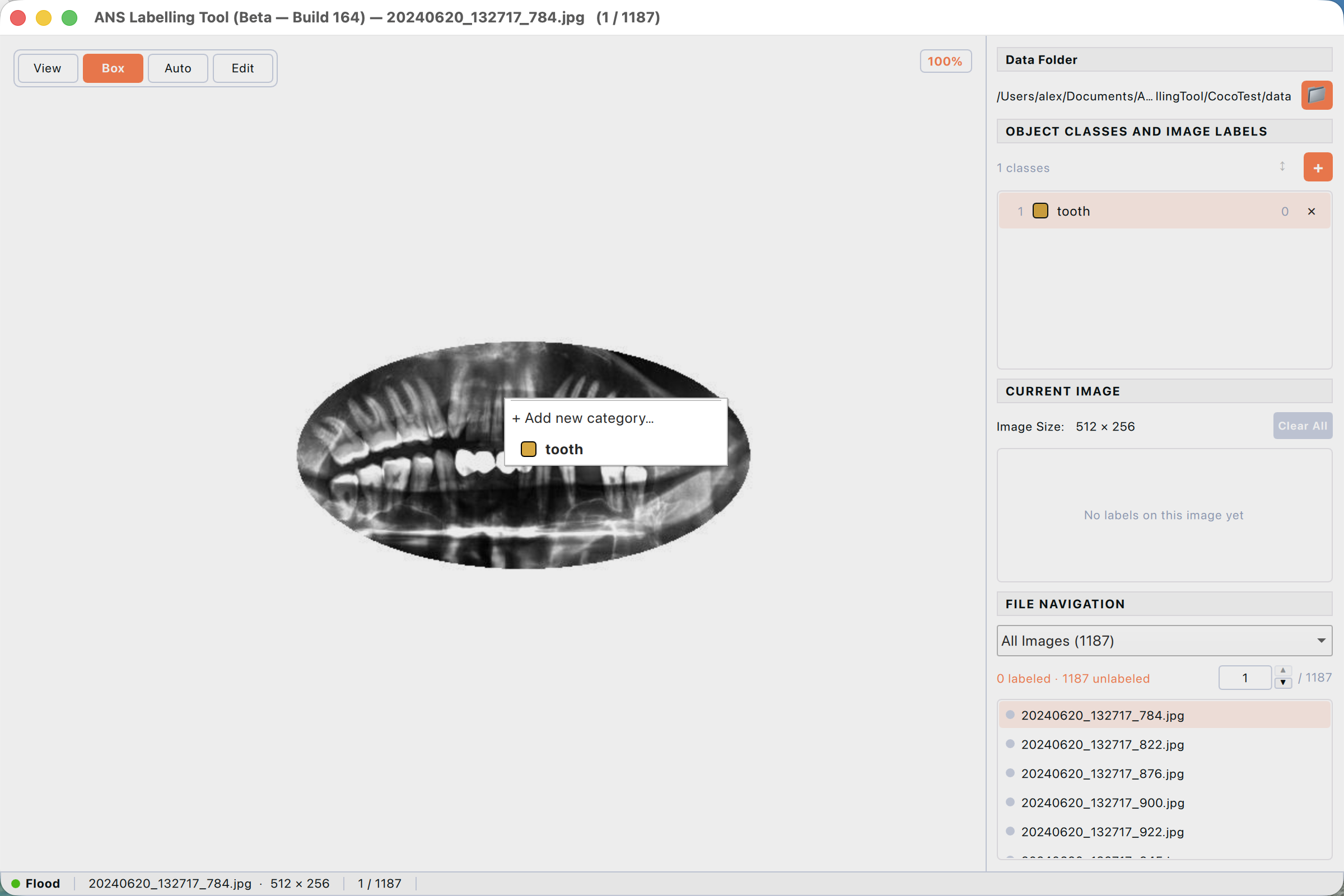
Figure: The label picker pops up at the release point. The current right-panel selection is shown in bold; “+ Add new category…” is always at the top.

Repeat for every visible object. The right panel’s Current Image section lists each label you commit. The grey dot in the file list flips to green as soon as the file has at least one label, and the counter at the bottom updates from “0 labeled” to “1 labeled”, etc.

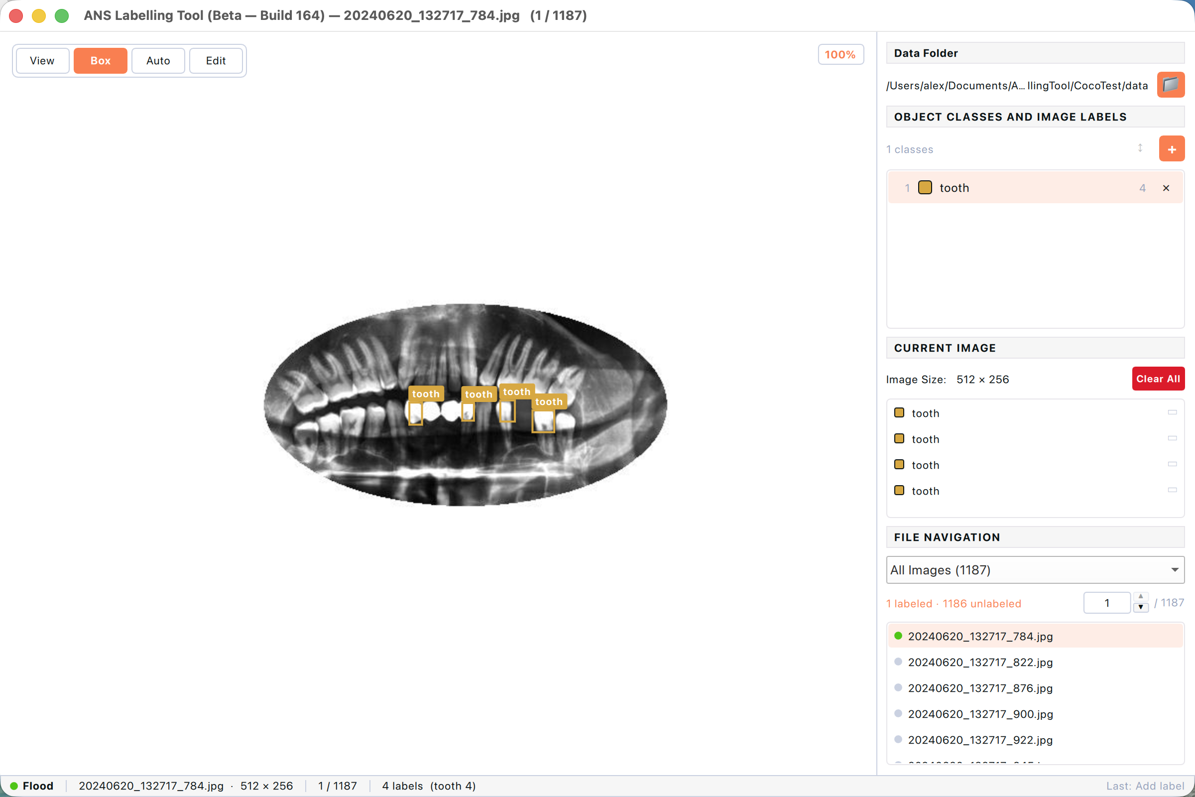
Figure: After four boxes have been committed, the right panel lists every label on the current image and the file list shows a green dot.

tip

there is no Save button. Labels are written to disk the moment you commit them, in the matching .txt sidecar (YOLO format). You can quit the app at any point without losing work.

8. Working through a dataset

Annotation is repetitive by nature. The file list and shortcuts below are designed so you almost never need to reach for the mouse to move between images.

8.1 File navigation panel

The bottom of the right panel lists every image in the dataset folder.

• The drop-down filters the list — All Images, Labeled, or Unlabeled.
• The numeric input next to the filter lets you jump to a specific row (1-based).
• Green dots mark labeled images, grey dots unlabeled. Click any row to load that image.
• Click the X unlabeled link in the counter to open a focused list of every remaining unlabeled file.

8.2 Navigating between images

Two equivalent ways to move:

• Press ⌘↓ for the next image and ⌘↑ for the previous one. The shortcut works regardless of which panel has focus.
• Click any row in the file list. The selected file scrolls into view in the list and renders in the canvas.

8.3 Copy / paste labels

If the next image is similar to the current one (a video frame, a slightly different angle), copy the labels and paste them onto the new image — then nudge in Edit mode.

1. On the source image, press ⌘C (or Edit → Copy labels).
2. Move to the destination image with ⌘↓ or by clicking it.
3. Press ⌘V (or Edit → Paste labels). Every copied label lands at the same canvas position.
4. Switch to Edit mode to drag any label that needs to be repositioned.

8.4 File context menu

Right-click any row (or multi-selection) in the file list to open a context menu with common dataset-management actions.

8.4.1 Selecting one or many files

The file list supports the same selection idioms as Finder / Explorer. You almost always act on more than one file — for example, augmenting a batch of similar frames or moving a subset to a held-out validation folder.

• Click a row — selects just that file and loads it in the canvas.
• ⌘-click (Ctrl-click on Windows/Linux) — adds or removes a single row from the existing selection.
• ⇧-click — selects every row between the previously clicked row and the shift-clicked one (range select).
• ⌘-A — selects every file currently visible in the filter (All / Labeled / Unlabeled).

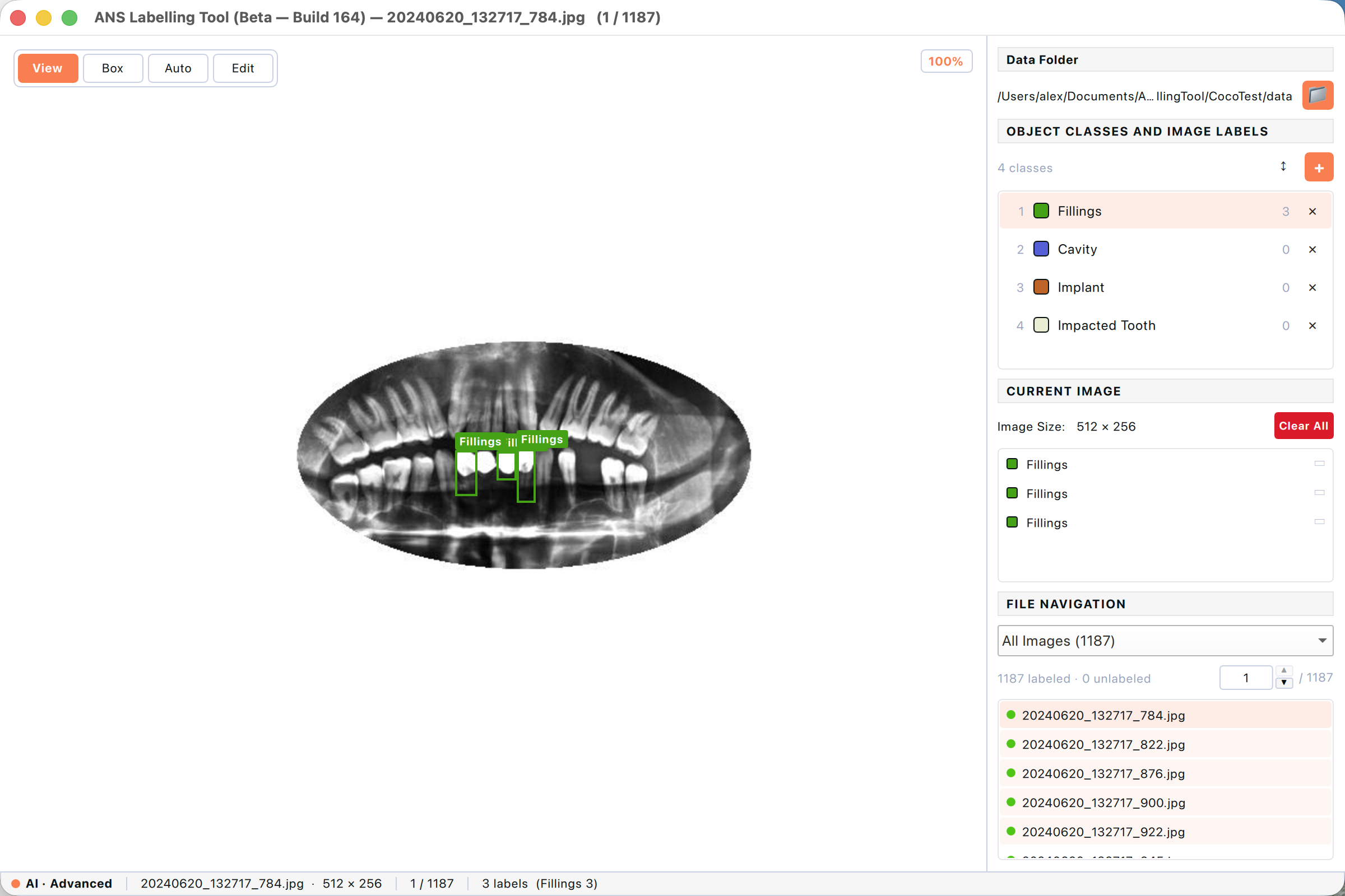
Figure: Multiple file rows highlighted in the right-panel file list. The orange row is the current image on the canvas; the others are part of the selection.

8.4.2 The right-click context menu

With one or more rows selected, right-click anywhere on the highlighted set to open the context menu. The first line of every action shows how many files it will operate on, so there’s no doubt about scope.

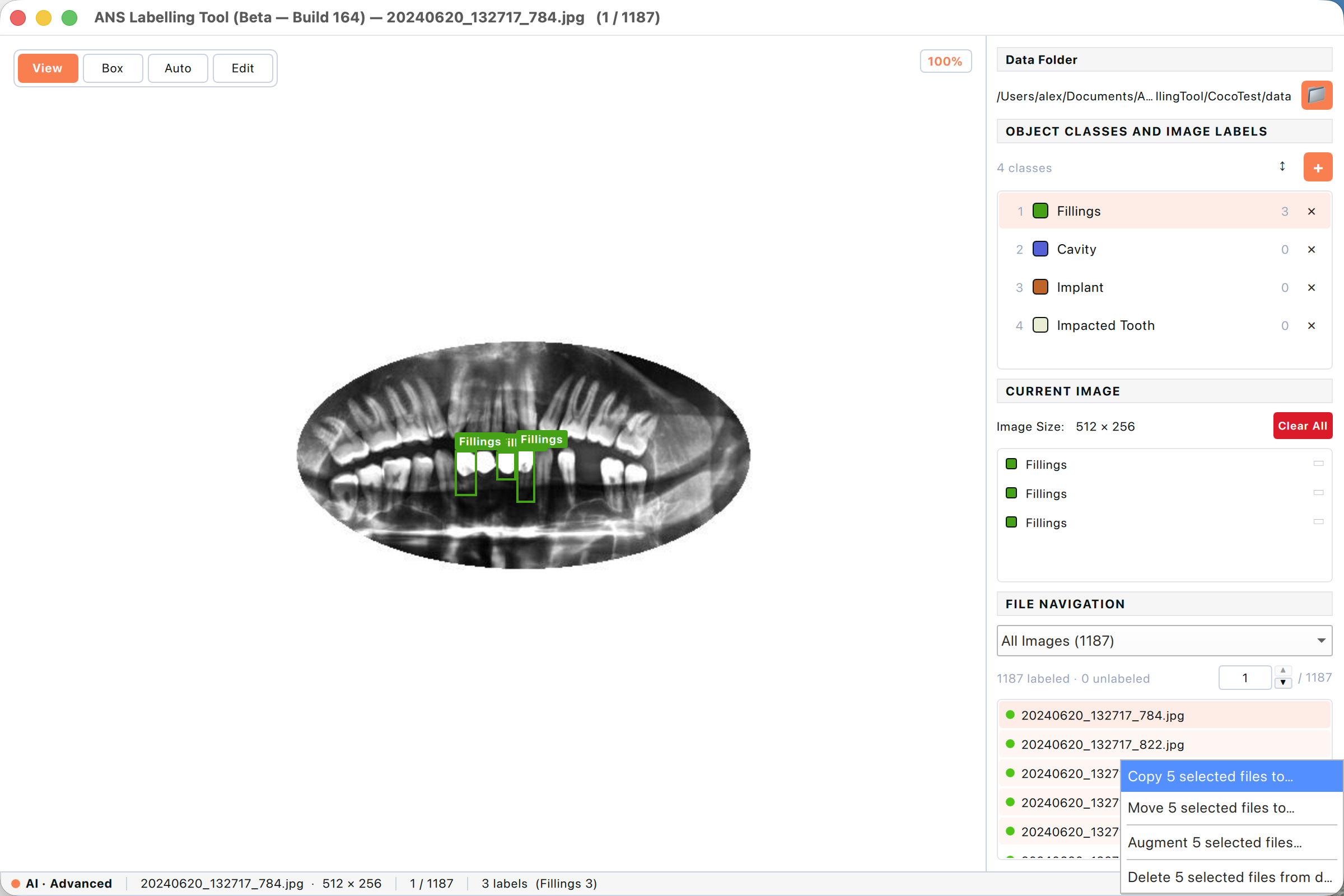
Figure: The file-list context menu after right-clicking a multi-file selection. Each entry includes the count (e.g. “Augment 5 selected files…”).

• Copy to… — copy the selected images plus their .txt sidecars to another folder, preserving labels.
• Move to… — same as Copy but removes the originals.
• Augment… — open the augmentation dialog (rotation, flip, brightness…) to produce new training images.
• Delete — move the selected images and labels to the system trash. Confirms first.

9. Power features

9.1 The Auto tool — Flood, AI Standard, AI Advanced

The Auto tool (press A or click Auto in the toolbar) speeds up labelling by letting you commit a shape with a single click on the object, instead of drawing it by hand. It has two backends and, inside the AI backend, two model tiers.

9.1.1 Flood backend

The Flood backend is a classic colour-similarity flood-fill. It is fast, runs entirely on CPU, and is well suited to objects with a uniform appearance on a contrasting background (circuit-board components, fruit on a tray, X-ray teeth). It does NOT understand object categories — only colour.

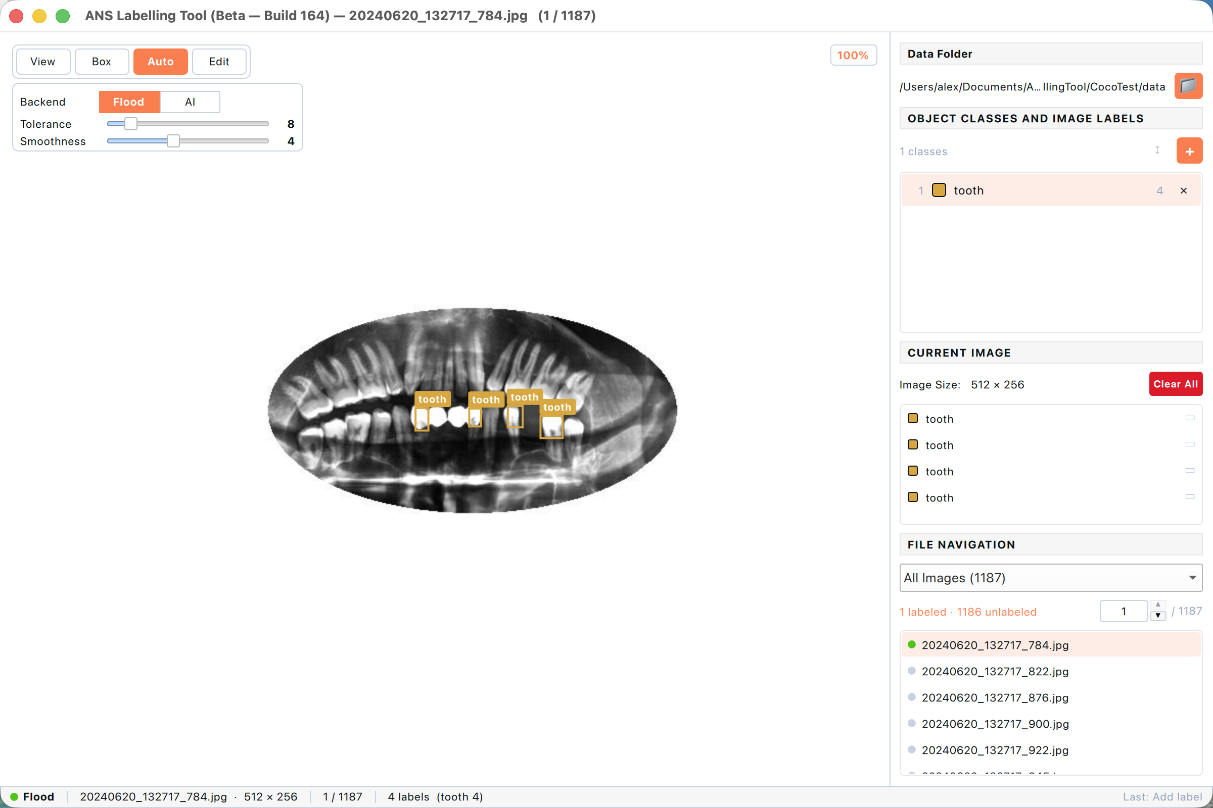
Figure: Flood backend selected. The panel shows two sliders: Tolerance (how lenient the colour match is) and Smoothness (how aggressively the resulting outline is simplified).

• Tolerance — higher values widen the colour range considered “same as the click”. Too high and the fill leaks into the background; too low and the fill stops at every shadow.
• Smoothness — how much the resulting outline is denoised. Higher = fewer vertices and cleaner polygons; lower = sharper edges but more vertex chatter.
• Backend is the right choice when there is no AI model available and the dataset has high colour contrast.

9.1.2 AI backend — Standard mode

Switching the Backend toggle to AI replaces the colour fill with a deep-learning segmenter. Standard mode uses Meta’s SAM 2.1 (Segment Anything Model) — about 200 MB, shipped inside the .app bundle, available offline immediately on first launch.

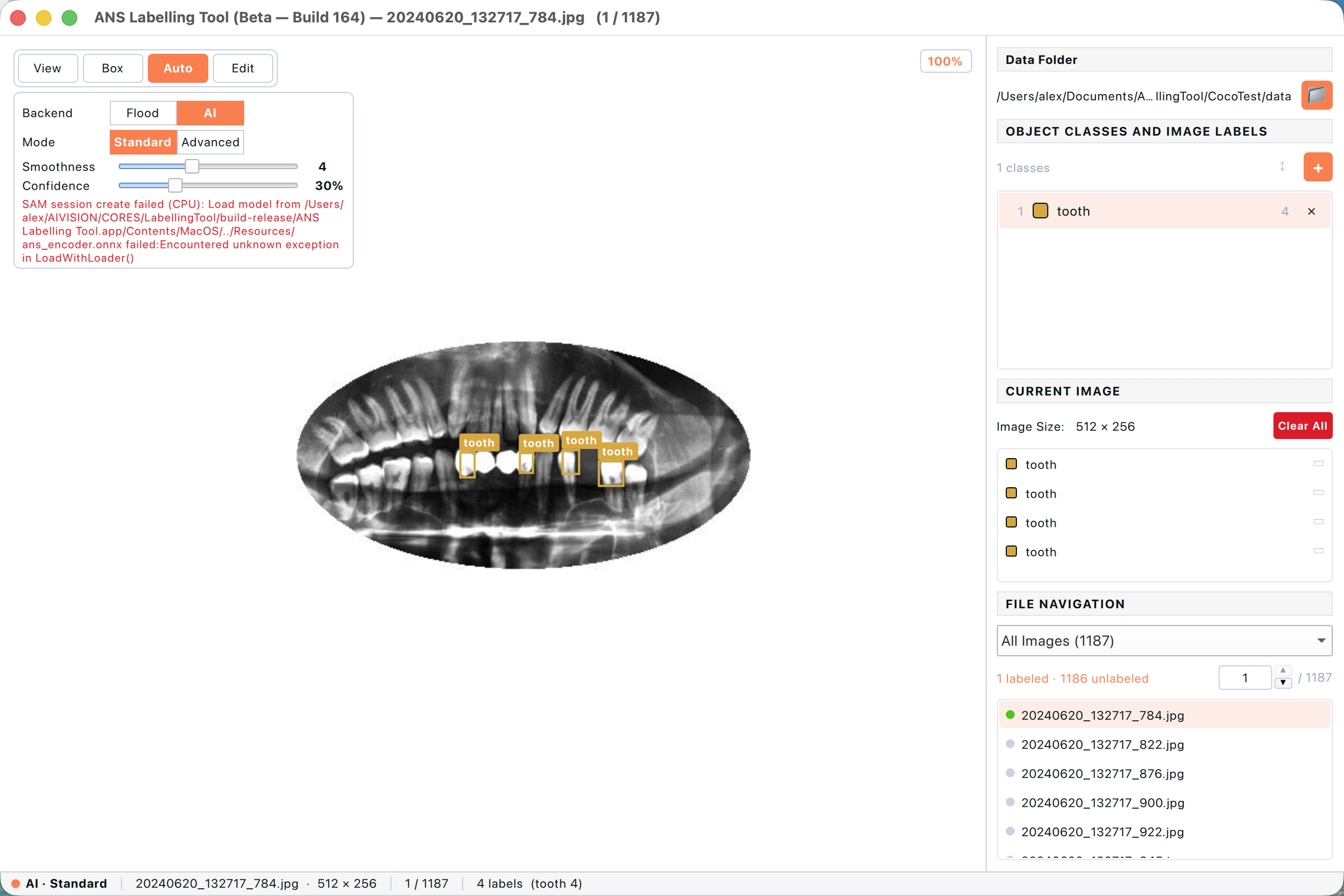
Figure: AI backend with Standard mode active. The Smoothness slider controls outline simplification; Confidence is the model’s minimum probability for the suggested mask.

• Smoothness — same as in Flood mode; controls polygon simplification.
• Confidence — minimum probability the model assigns to its suggested mask. Below this threshold the suggestion is skipped.
• Status bar shows “AI · Standard” while this mode is active.
• Works fully offline — no network needed.

9.1.3 AI backend — Advanced mode (SAM 3)

Advanced mode uses Meta’s SAM 3 — significantly more accurate than Standard, especially on small, occluded, or unusually-shaped objects. The model is large (≈ 3.4 GB) and is NOT bundled with the app to keep the installer small. The first time you select Advanced, the tool offers to download it for you.

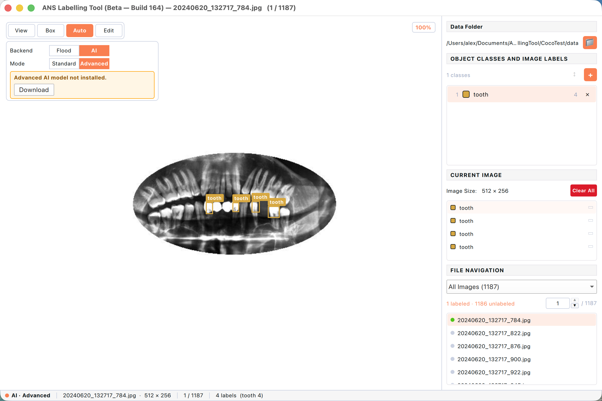
Figure: Advanced mode selected for the first time. A banner reads “Advanced AI model not installed” with a Download button. Standard mode keeps working in the background.

1. In the Auto panel, set Backend → AI and Mode → Advanced.
2. If the banner “Advanced AI model not installed.” appears, click Download. The app fetches the SAM 3 model archive (~3.4 GB) into a shared folder managed by the tool.
3. A progress indicator shows download status. Cancel and resume are both supported.
4. Once the download finishes the banner disappears and Advanced sliders take effect (Confidence, plus a text-prompt picker for SAM 3’s “anything can be prompted” mode).

note

the SAM 3 download is one-time per machine. Multiple user accounts on the same computer share the model file. If your machine is offline or behind a strict firewall, your IT team can install the model archive manually — the tool will detect it on the next launch.

9.2 Auto-label

Auto-label runs a pre-trained ANS model over the entire dataset folder and writes the predicted labels as .txt sidecars. Use it as a starting point — you still need to review and correct, but you may save hours on large datasets.

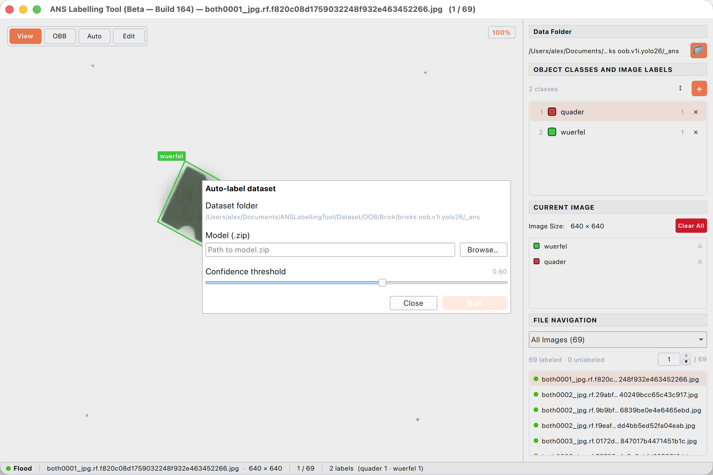
Figure: Auto-label dialog. Pick a model and a confidence threshold, then click Run.

1. Choose File → Auto-label…
2. Click Browse and pick a .zip model file (the ANS model archive supplied for your dataset).
3. Adjust the Confidence threshold slider. Higher values mean fewer false positives but more missed objects.
4. Click Run. A progress bar appears in the dialog and the status bar; the run can be cancelled at any time.
5. When it finishes, the labels are written to disk and immediately visible in the file list and canvas.

note

Auto-label overwrites any existing .txt sidecars for the predicted images. If you have hand-corrected labels you want to keep, back up the folder first.

9.2.1 Worked example — full dataset auto-label

The following walk-through uses the included CocoTest dental dataset (1,187 X-ray images) and the supplied ANS_TestCoco(GPU)_1.zip model. The model is trained to detect four dental classes — Cavity, Fillings, Impacted Tooth, and Implant. Auto-label will create those classes automatically and write a .txt sidecar for every image.

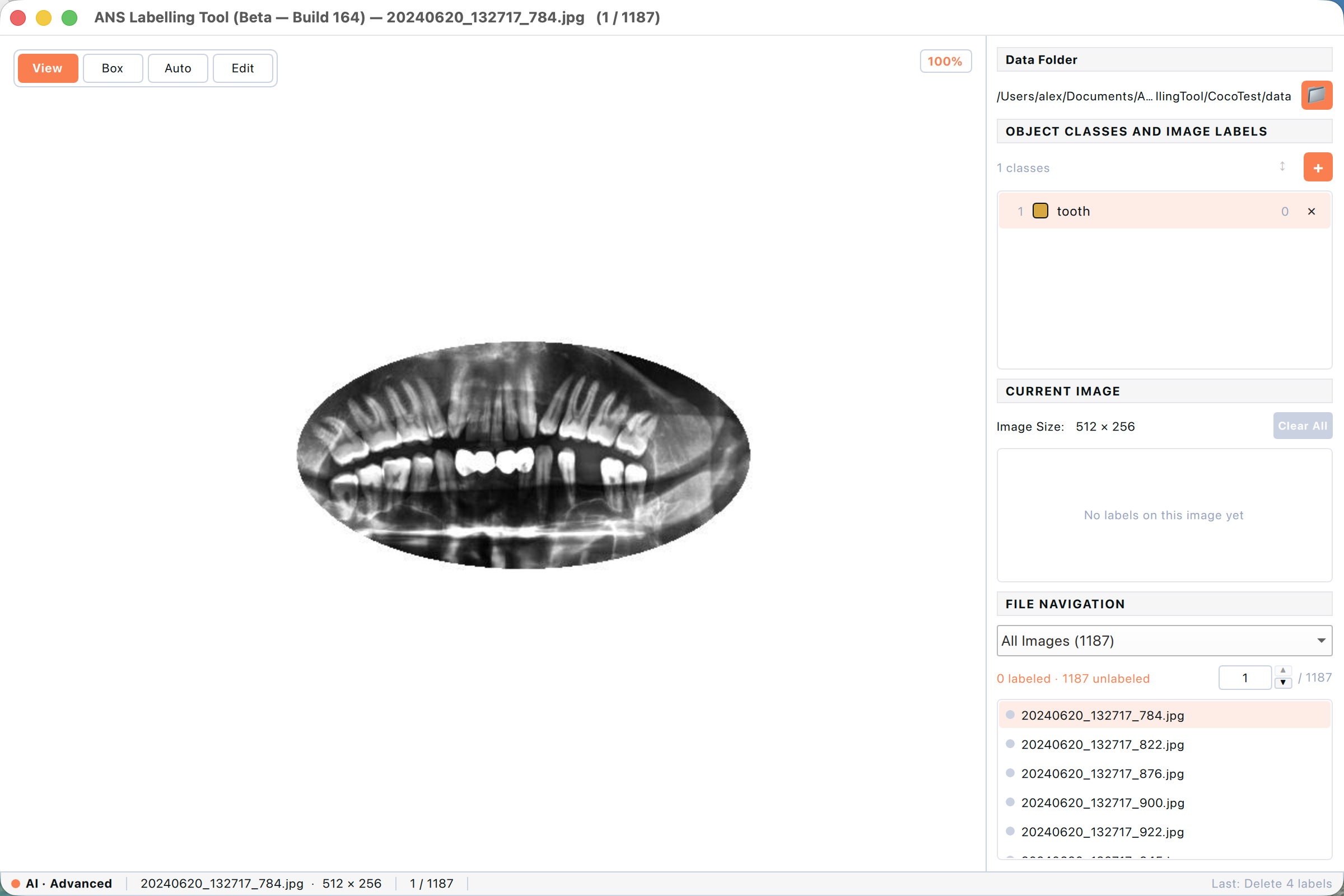
Figure: A freshly opened CocoTest folder. 1,187 unlabeled images, no categories defined yet.

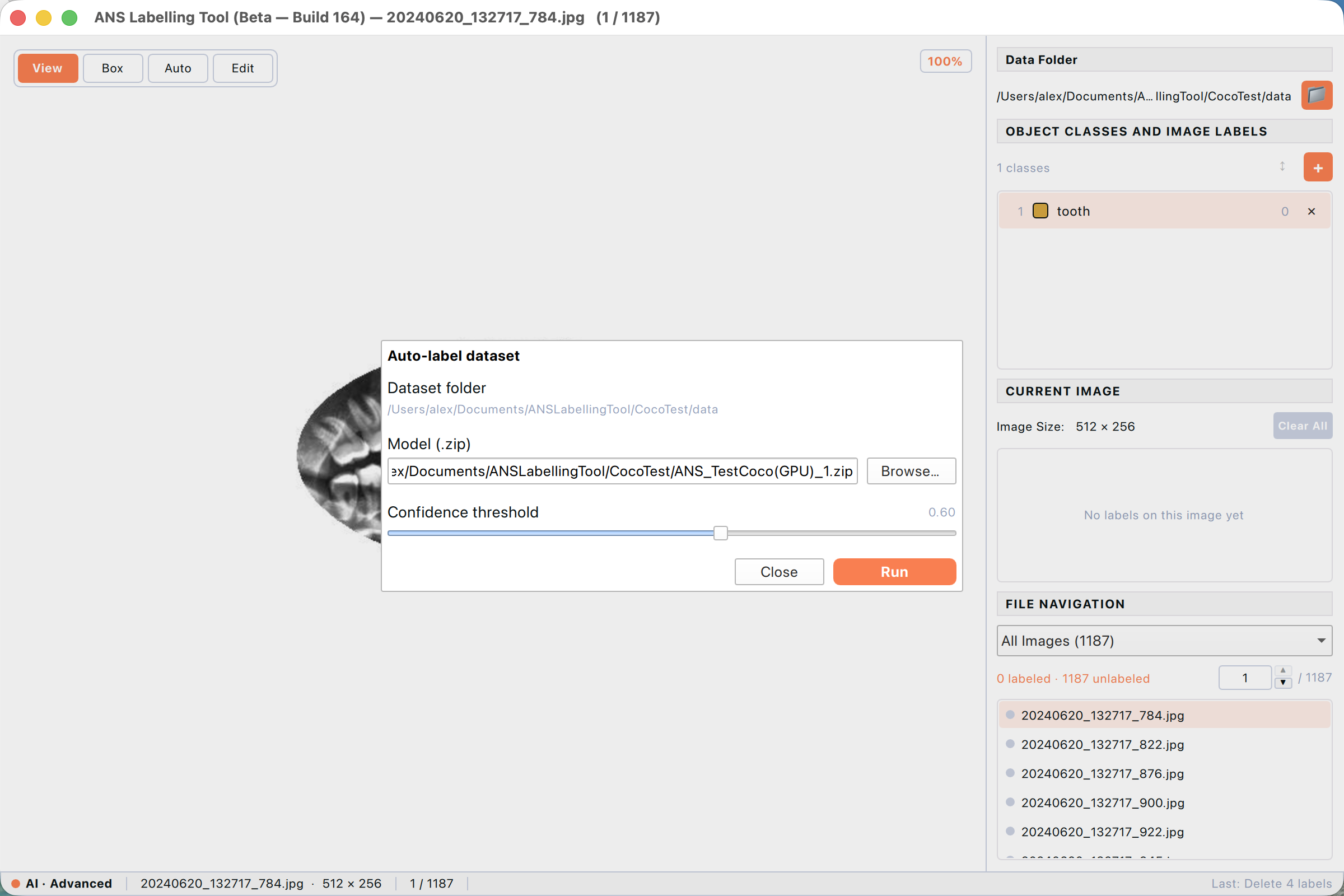
Figure: Auto-label dialog with the model archive selected and a confidence threshold of 0.60. Run lights up once a valid model is chosen.

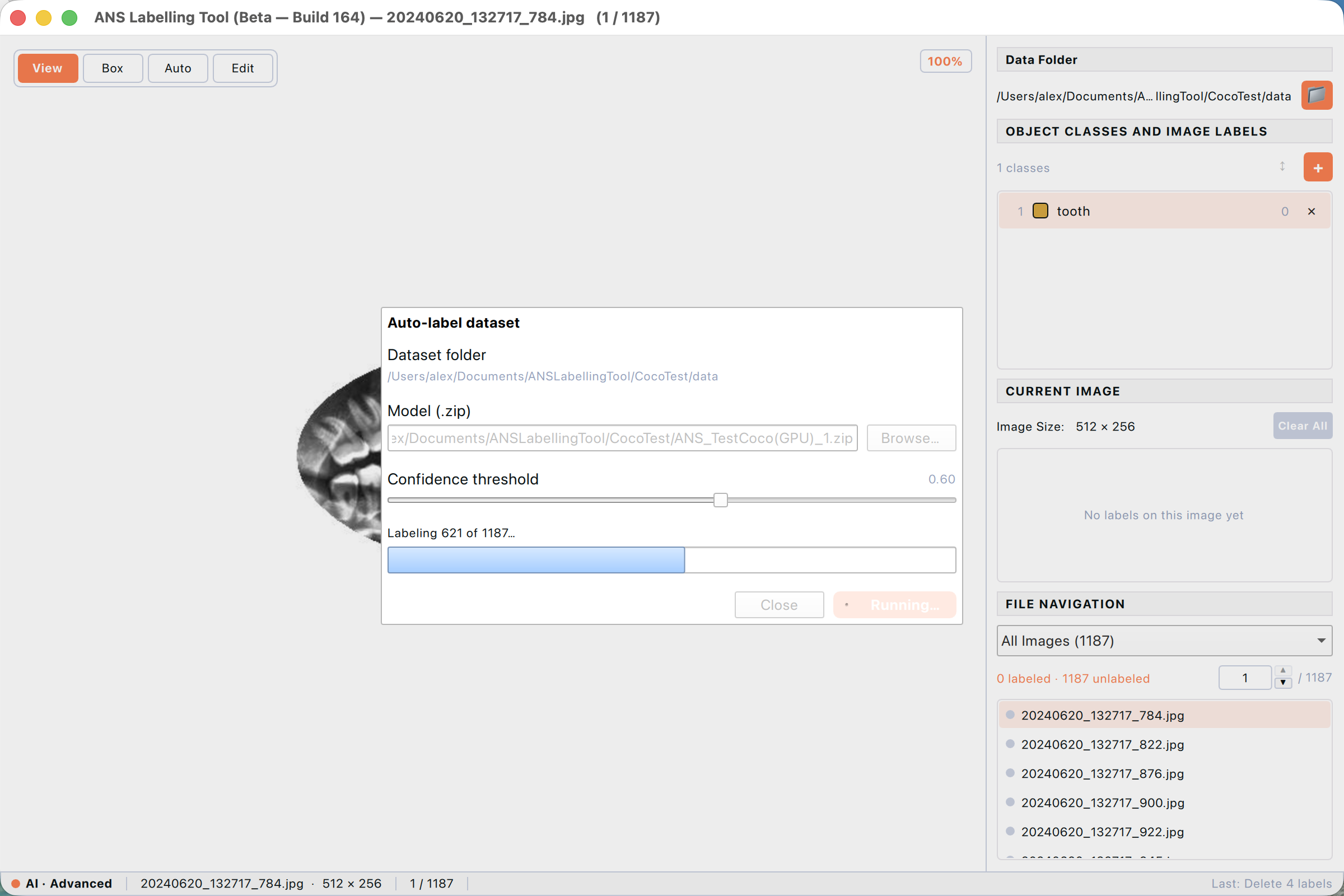
Figure: Mid-run progress — the model labels each image in turn. The Run button is replaced by a stop indicator; you can Close to cancel.

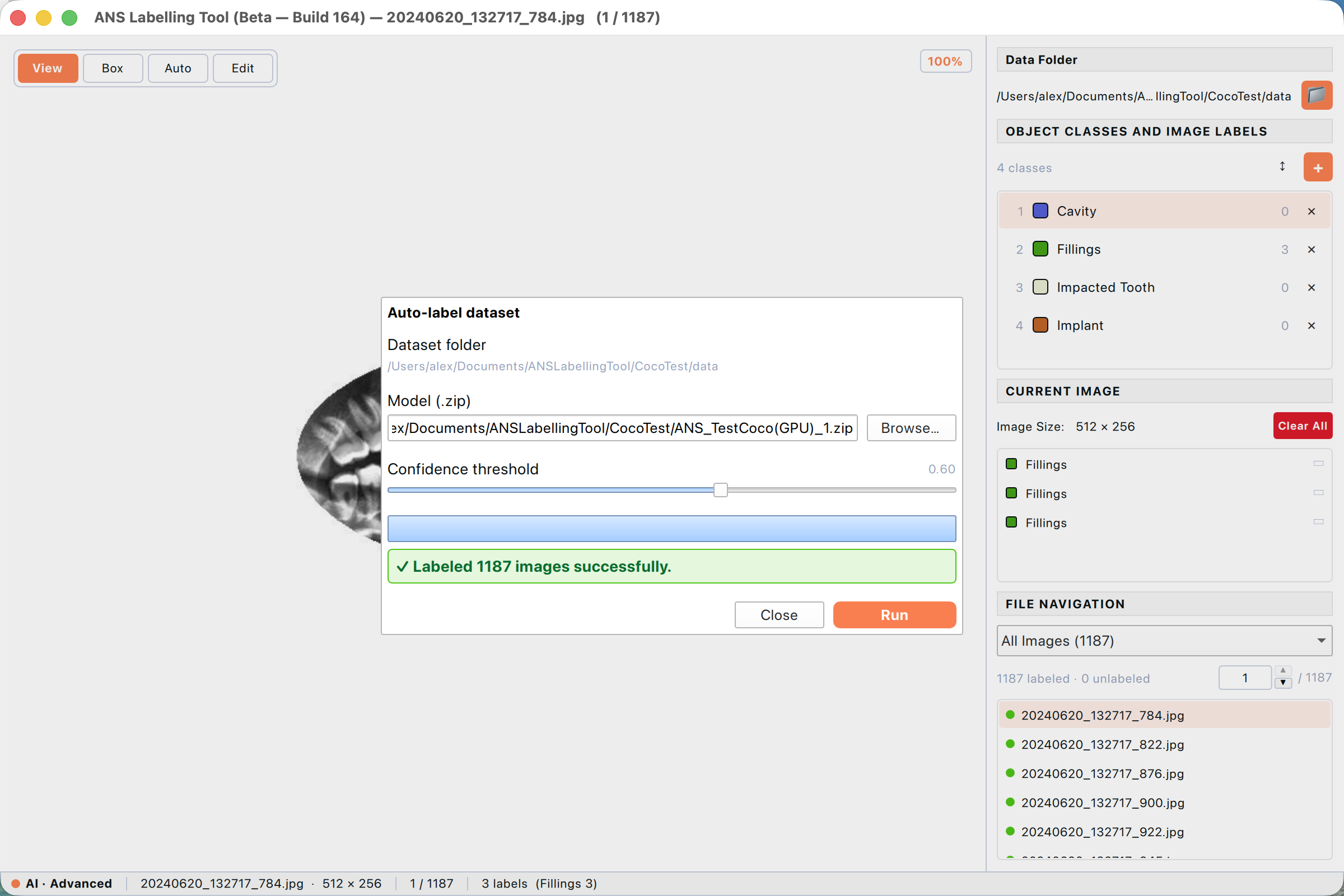
Figure: After ~1–2 minutes (GPU), the banner reports “Labeled 1187 images successfully” and the four model classes (Cavity, Fillings, Impacted Tooth, Implant) appear in the right panel.

Figure: Returning to the canvas you see the predicted boxes (Fillings in green here) overlaid on the X-ray. Every file in the list now has a green dot — 1,187 labeled, 0 unlabeled.

From here you would normally walk every image (⌘↓), spot-check the predictions, and use Edit mode to correct any wrong boxes or add ones the model missed. The model gives you a head start — usually 80–95% of the work is already done.

9.3 Rearranging categories

The order of categories in ANS_Class.json determines the class index in every .txt sidecar. After Auto-label or after adding many classes by hand, you may want to reorder them to match the order your training pipeline expects.

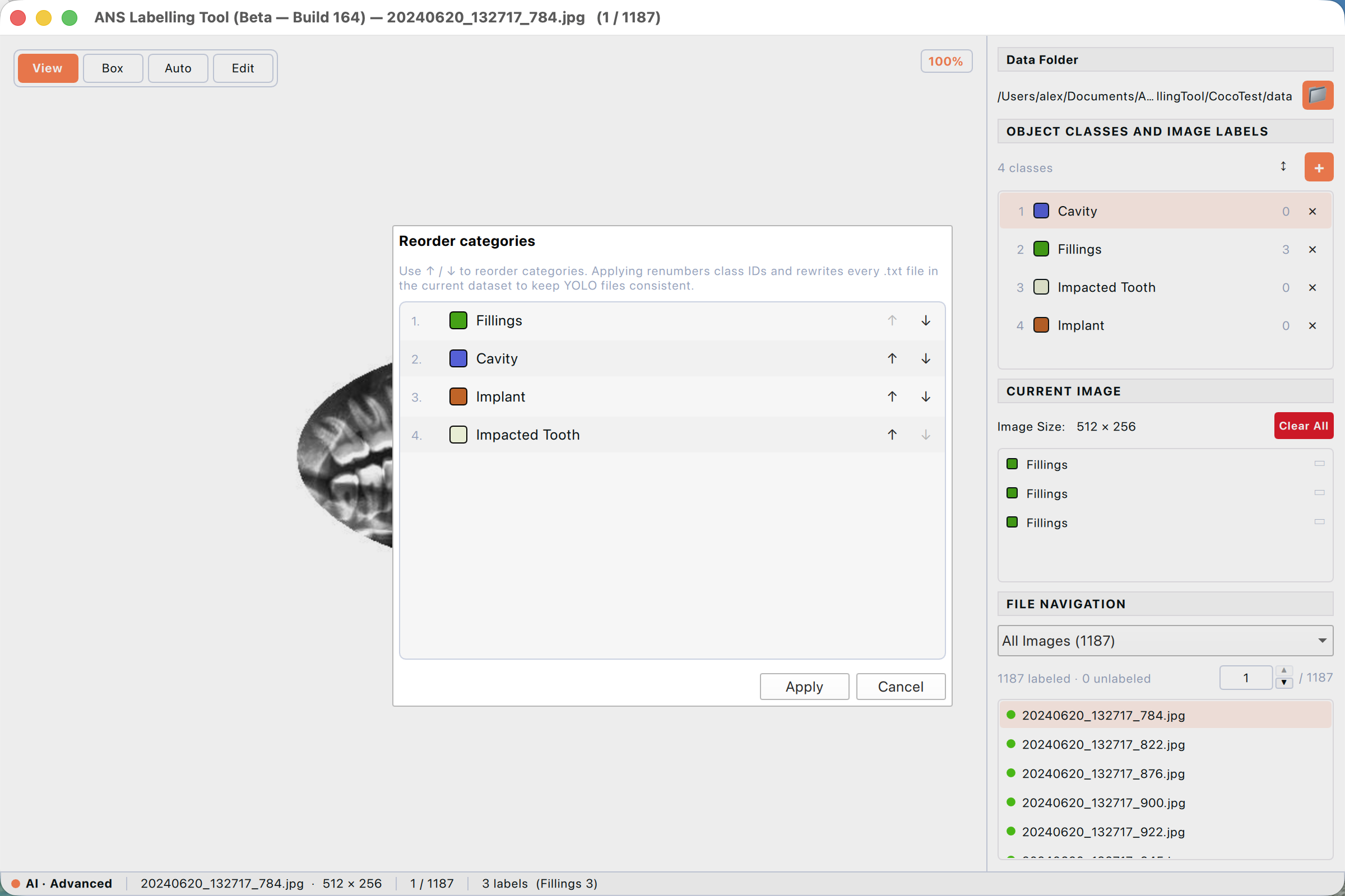
Figure: The Reorder categories dialog. Each row has up/down arrows to move it. The warning at the top reminds you that Apply rewrites every .txt file in the dataset.

1. Click the ↕ icon in the top-right of the Object Classes and Image Labels header — between the title and the orange + button.
2. The Reorder categories dialog appears.
3. Use the ↑ / ↓ arrows beside each row to move that category up or down.
4. Click Apply to commit. The tool renumbers the class IDs in ANS_Class.json and rewrites every .txt sidecar to use the new IDs — your dataset stays consistent.
5. Click Cancel to discard the changes.

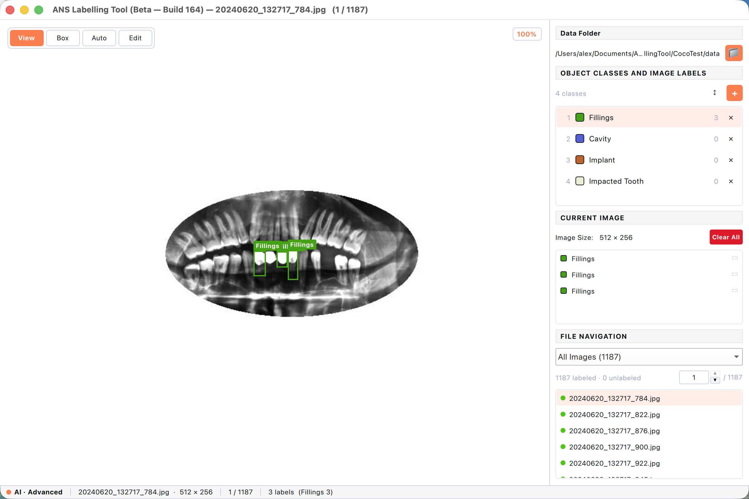
Figure: After Apply, the right-panel category list reflects the new order with renumbered IDs (1, 2, 3, …). Existing boxes on every image keep their visual mapping to the right class.

note

Apply rewrites every .txt sidecar — for large datasets this can take a few seconds. There is no undo for this operation; the change is committed straight to disk. The visual appearance of every label on every image is preserved.

9.4 Dataset statistics

View → Dataset statistics… opens a per-category breakdown of the entire dataset: total images, total labels, count per class, and the percentage share. Use it to check class balance before training — most modern detectors struggle when one class has 90× more instances than another.

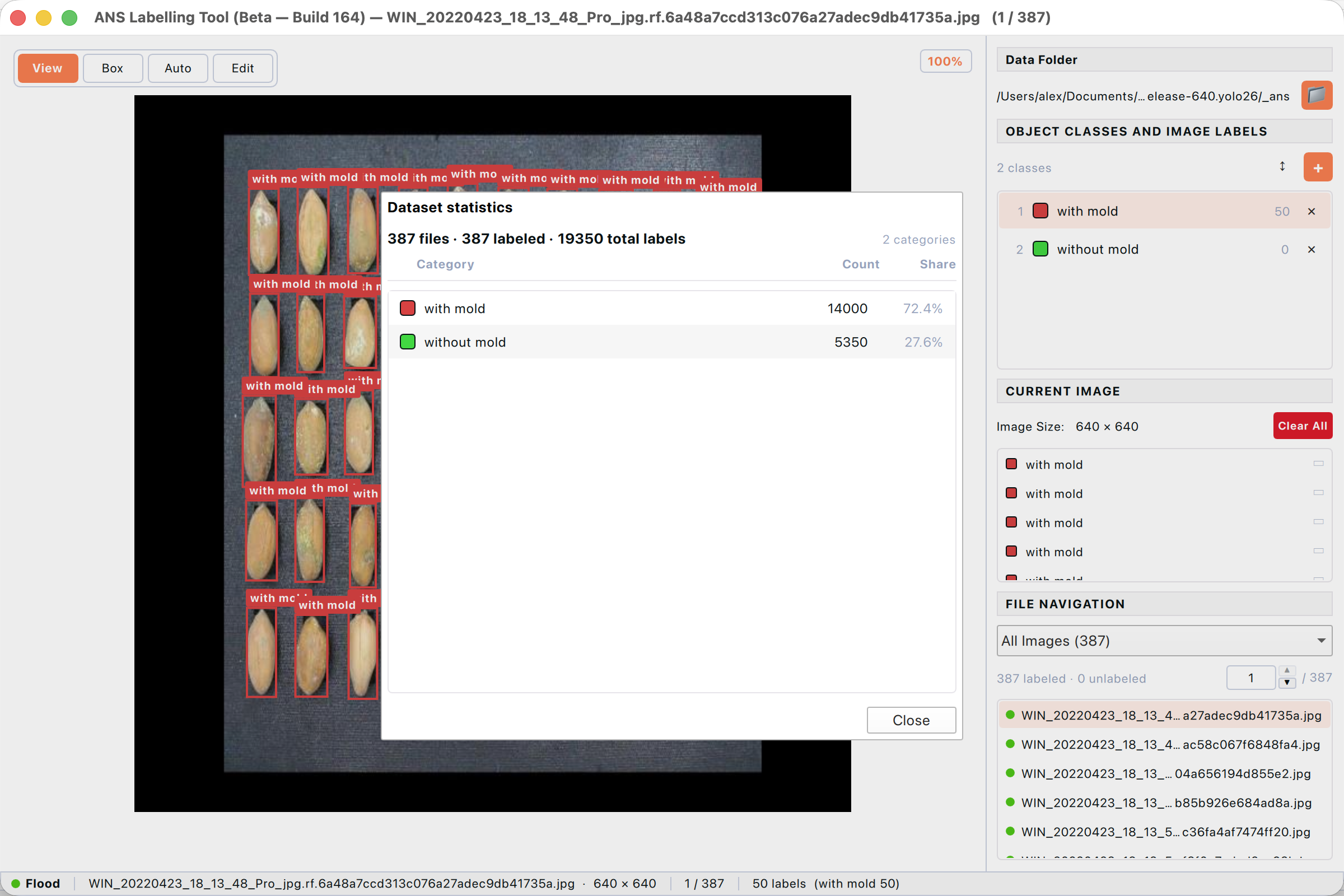
Figure: Dataset statistics showing per-class counts and the percentage share.

9.5 Switching annotation task

File → Switch task… reopens the same picker you saw on first launch. The app remembers the most-recent dataset folder per task, so switching back is instant.

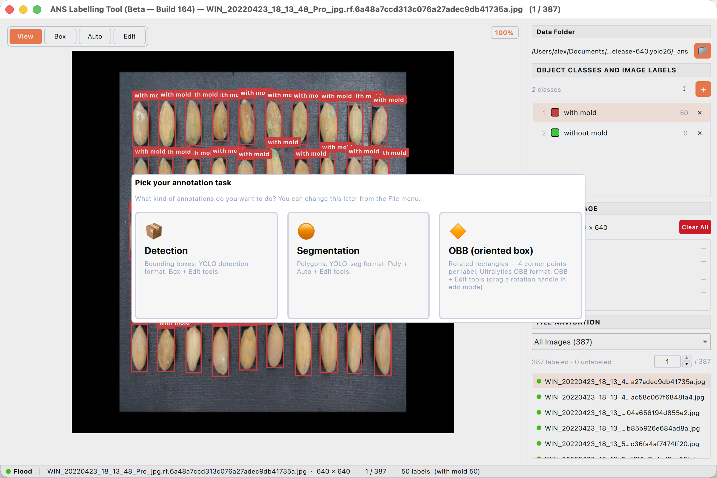
Figure: The Switch task dialog opened from File → Switch task… It is the same picker as on first launch.

9.6 Image augmentation

Right-click a file (or selection) and choose Augment… to generate new training images from your annotated ones. Available transformations include:

• Horizontal flip and vertical flip.
• Rotation in 90° steps.
• Brightness and contrast adjustments.
• Each combination produces one new image with all label coordinates correctly transformed.

9.6.1 The Augment dialog at a glance

Right-click → Augment… opens a dedicated dialog tailored to bulk transformation. It is designed so you can preview the exact output before any file is written to disk — useful for spotting weird interactions between transforms (e.g. a blur that erases small labels).

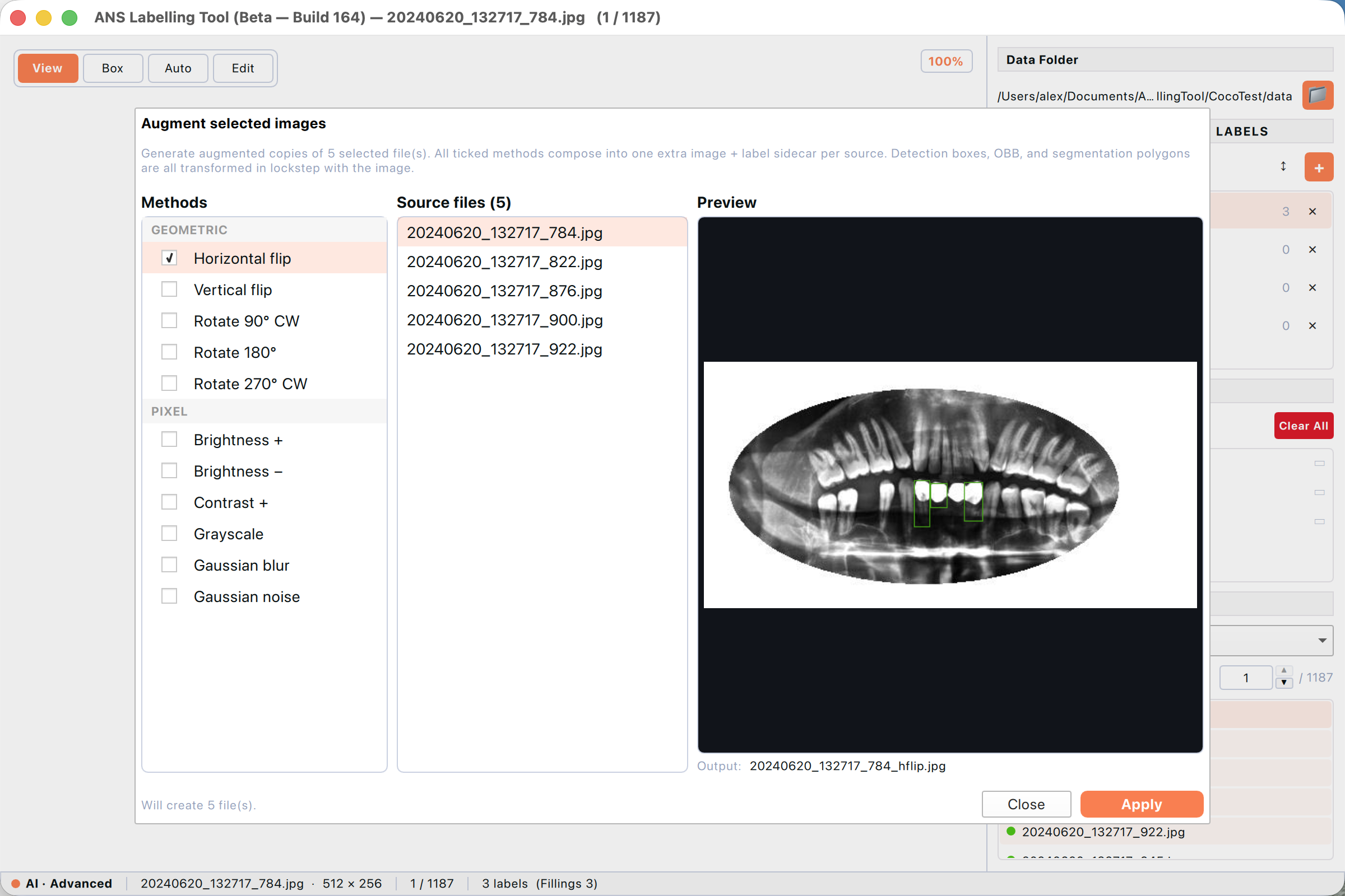
Figure: The Augment dialog with Horizontal flip ticked. Three panes — Methods (left), Source files (centre), live Preview (right) showing the flipped image with the green Fillings labels mirrored correctly. The Output filename below the preview previews the suffix chain.

• Methods — every available transform grouped by category (GEOMETRIC: flips, rotations; PIXEL: brightness, contrast, grayscale, blur, noise). Tick each method you want applied.
• Source files — the list of files the right-click selection passed in. Click any row to focus the preview on that file. Clicking here does NOT change which files get processed — Apply still runs on the entire list.
• Preview — a live rendering of the focused source file with every ticked method applied in catalogue order. Detection boxes, OBBs and segmentation polygons are transformed lockstep with the pixels, so the preview shows exactly what the saved label sidecar will contain.

9.6.2 Composing multiple methods

When you tick more than one method, the dialog composes them into a single output image per source — they are NOT generated as separate files. Geometric transforms run first, then pixel transforms. The output filename includes a suffix for every method in order so you can read the chain from the filename alone.

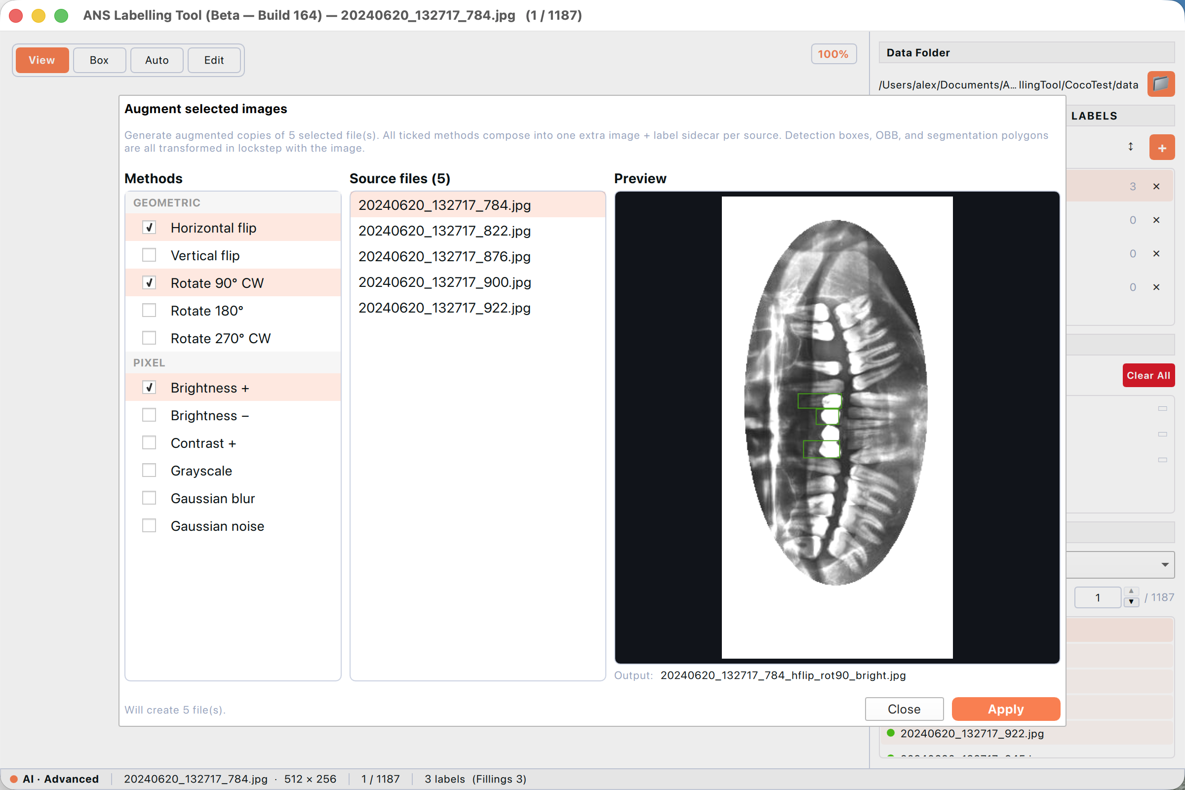
_Figure: Three methods ticked — Horizontal flip + Rotate 90° CW + Brightness +. The preview shows the composed result; the Output filename reads “…hflip_rot90_bright.jpg”. Status at the bottom-left reports how many files will be created.

1. Tick every method you want applied. Use the preview to confirm the composed result looks right.
2. Click any Source file to spot-check that the same composition works on different inputs.
3. Check the “Will create N file(s).” count in the bottom-left to confirm the scope.
4. Click Apply. The tool writes one new image (+ matching .txt sidecar) per source into the dataset folder, with the suffix chain in the filename.
5. On success the dialog auto-closes and the new files appear in the file panel (they share the same labelled / unlabelled dot logic as the originals). Failures keep the dialog open so you can read the warning.

tip

Augment is destructive in the sense that it writes new files — but never modifies the originals. If you change your mind, delete the augmented files via the same right-click menu (they all share the suffix you chose). The labels stay in lockstep because the same transform is applied to both pixels and label coordinates.

10. Display preferences

View → Display preferences… controls how labels look on the canvas. These settings are stored per user and apply globally — they do not change the data on disk.

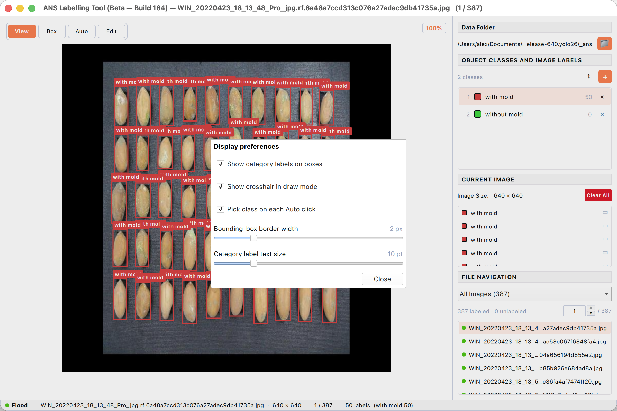
Figure: Display preferences — control how labels are rendered on the canvas.

• Show category labels on boxes — toggle the small text badge attached to each label. Useful to turn off when boxes overlap heavily.
• Show crosshair in draw mode — the thin horizontal/vertical guides that track the cursor while drawing. Helpful for precise alignment.
• Pick class on each Auto click — controls whether the category picker appears after each Auto-segment commit. Turn off for batch labelling of one class.
• Bounding-box border width — 1 to 6 px. Higher values are easier to see on busy images.
• Category label text size — 8 to 18 pt for the small class badges.

11. Keyboard shortcuts

All shortcuts can also be opened in the app via Help → Keyboard shortcuts… (or press ?).

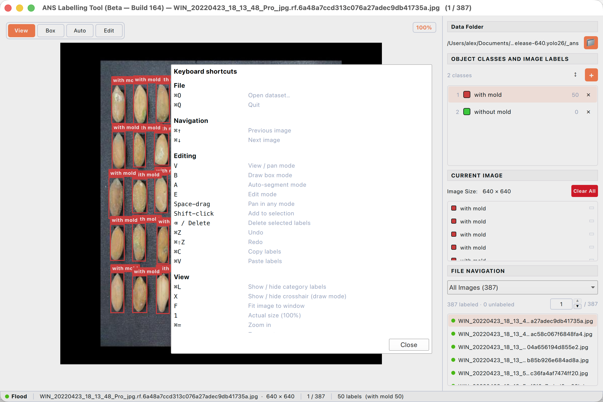
Figure: Built-in keyboard shortcut reference — opens with ? from anywhere in the app.

11.1 File

Shortcut	Action
⌘O	Open dataset
⌘Q	Quit the app

11.2 Navigation

Shortcut	Action
⌘↓	Next image
⌘↑	Previous image

11.3 Editing

Shortcut	Action
V	View / pan mode
B	Draw box mode (detection)
P	Draw polygon mode (segmentation)
O	Draw OBB mode (oriented box)
A	Auto-segment mode
E	Edit mode
Space + drag	Pan in any mode
⇧ + click	Add to selection
⌫ / Delete	Delete selected labels
⌘Z	Undo
⌘⇧Z	Redo
⌘C	Copy labels
⌘V	Paste labels
R (hold)	Rotate OBB while drawing

11.4 View

Shortcut	Action
⌘L	Show / hide category label badges
X	Show / hide draw-mode crosshair
F	Fit image to window
1	Reset zoom to 100%
⌘= / ⌘+	Zoom in
⌘−	Zoom out
⌘ + scroll	Zoom at cursor
Scroll	Pan vertically
⇧ + scroll	Pan horizontally
?	Open Keyboard shortcuts dialog

12. Troubleshooting

Common issues and how to resolve them. If you hit something not covered here, email support@anscenter.com with the screenshot and a description.

Q: Sign In button stays disabled.

A: The button only enables when both Email and Password contain something. Check for stray spaces; the email is automatically lower-cased so capitalisation is not the issue.

Q: I get “Invalid credentials” but my password is right.

A: Reset your password from the ANSCENTER portal (https://portal.anscenter.com.au). If your account is new it may still be pending admin approval.

Q: Open Dataset… does nothing or shows an empty file list.

A: The folder you chose has no images in a supported format. Open the folder in Finder and confirm there are .jpg / .jpeg / .png / .bmp files. If the folder is in YOLO / COCO / VOC format, the Import dataset dialog should appear instead — if it doesn’t, the folder is missing the expected structure (e.g. a yolo dataset without data.yaml).

Q: Labels appear at the wrong place after I rotate or augment an image.

A: This usually means the image was rotated externally (e.g. in Preview) after labels were saved. Re-open the dataset, redraw the affected labels, and the geometry will match again. Augment inside the app always keeps label coordinates consistent.

Q: Auto-segment shows “Backend unavailable”.

A: The AI backend needs the SAM model files (downloaded automatically on first use). If the download was blocked, you can fall back to the simpler Flood-fill backend from the right-side Magic panel — it works without GPU.

Q: The app warns about NVIDIA CUDA on launch.

A: On Windows / Linux with an NVIDIA GPU, the app expects CUDA + cuDNN libraries on PATH. The CUDA setup dialog walks you through installing the right driver and library files. On macOS the CUDA dialog never appears — Apple Silicon uses Metal automatically.

About the application

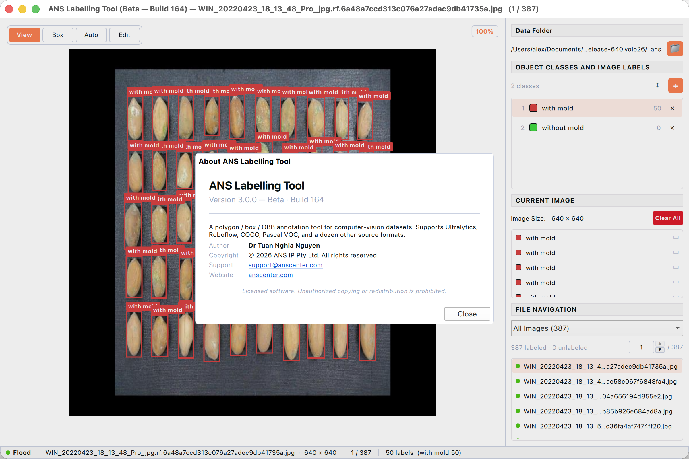
Figure: About dialog showing the app version, build, author and contact details.

Help → About… shows the running version, build number, the source-format list, and the support contact details. Quote the build number when reporting issues so support can match it to a release.

Licensed software — unauthorised copying or redistribution is prohibited.